Molecular Dynamics Simulations for Materials and Molecule Discovery - From Fundamental to Emerging Trends-

Molecular Dynamics Simulations –Transforming Materials and Molecules R&D–

Driven by remarkable advances in computational power in recent years, molecular dynamics (MD) simulations have become an indispensable tool in the research and development of materials, chemistry, drug discovery, and  biosciences. This method, which tracks the movement of individual atoms and molecules over time, offers a unique window into the fundamental processes of the physical world.

Often referred to as a “microscope with exceptional resolution,” MD simulations make it possible to visualize atomic-scale dynamics that are otherwise difficult—or even impossible—to observe experimentally. This capability provides deeper insights into the underlying mechanisms of complex physical and chemical phenomena, providing a foundation for rational materials and molecule design that goes beyond what can be achieved through experiments alone. Moreover, by enabling virtual testing across a wide range of conditions—such as temperature, pressure, and composition—MD simulations can significantly accelerate the overall R&D process by guiding experimental efforts more efficiently.

In this article, we will introduce the fundamentals and recent trends in molecular dynamics. We will also explore the diverse physical phenomena that can be analyzed using this powerful computational technique.

What Can We Observe with Molecular Dynamics Simulations?

MD simulations generate time-series data of atomic coordinates, velocities, energies, and other properties in a system. By analyzing these data appropriately, researchers can quantitatively evaluate key properties of the system under study and extract meaningful insights into its behavior.

In this section, we will explore several representative use cases and common analysis methods to illustrate how these simulation tools are applied in practice.

(1) Radial Distribution Function: Quantifying Structural Features

Unlike crystalline materials, the detailed atomic-level structures of liquids and amorphous materials are generally difficult to observe experimentally. Molecular dynamics simulation is a powerful tool to directly capture atomic configurations and dynamic behavior in such systems.

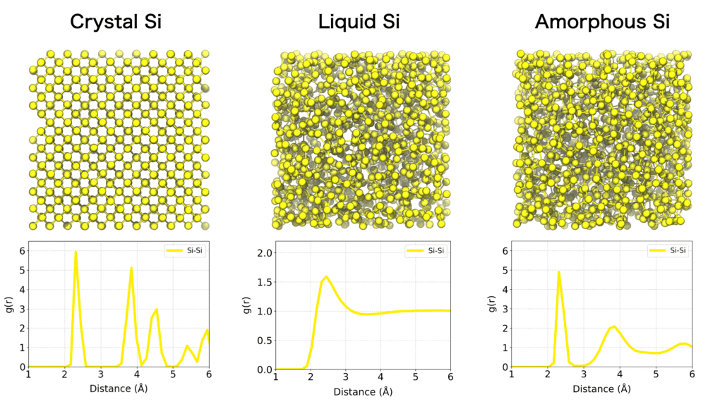
One of the most widely used methods for quantitatively characterizing the structure of materials is the radial distribution function (RDF). The RDF describes how atoms are spatially distributed around a reference atom as a function of radial distance r. It is particularly useful for analyzing both ordered systems, such as crystalline solids, and disordered systems like liquids and amorphous materials, which often exhibit local structural order.

By analyzing the RDF, one can quantitatively determine characteristic interatomic distances, such as those corresponding to the first and second coordination shells, as well as coordination numbers. The overall shape of the RDF also reflects the phase state of the system. For example: Crystalline solids exhibit sharp, periodic peaks corresponding to their long-range order. Liquids and amorphous materials display broader peaks indicative of short-range order, with the function gradually converging to 1 at larger distances. In the gas phase, where atomic interactions are sparse, the RDF remains close to 1 across all distances.

The RDF is also essential for validating simulation models, as it enables direct comparison with experimental data such as structure factors derived from X-ray or neutron diffraction. Accordingly, it is widely used to analyze a variety of systems and phenomena—including liquid and glass structures, solvation shells, and interfacial organization.

(2) Diffusion Coefficient: Quantifying the Mobility of Ions and Molecules: 

The diffusion of ions and molecules plays a vital role in determining the chemical and mechanical properties of materials—for example, ion conductivity in liquids, ion transport in solid electrolytes, and the diffusion of small molecules within polymers. MD simulations enable the direct observation of both the pathways and the rates at which these species move through a material.

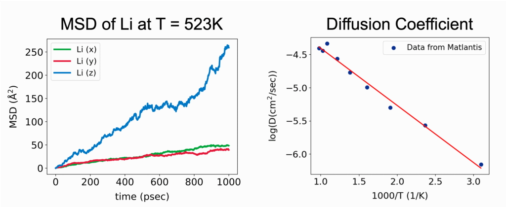
The movement of ions and molecules can be quantitatively characterized using the diffusion coefficient, a key metric for evaluating mobility. In the MD simulations, the diffusion coefficient is calculated from the time evolution of the mean square displacement (MSD). MSD represents the average squared displacement of particles over time. More precisely, it is defined as the average of the squared distance between a particle’s initial position, ri(0), and its position at a later time t, ri(t), taken over all particles and different initial time origins.

In the diffusive regime, where particles exhibit random-walk behavior over sufficiently long timescales, the MSD increases linearly with time. The slope of this linear region allows the diffusion coefficient D to be calculated based on Einstein’s relation. For a three-dimensional system, this relation is expressed as:

Evaluating the diffusion coefficient not only enables direct comparison between simulation and experimental results but also provides a quantitative understanding of transport mechanisms within materials. Moreover, by systematically varying parameters such as temperature, pressure, and composition, MD simulations allow researchers to explore the energy barriers that govern diffusion processes. These insights are invaluable for accelerating materials design and optimizing processing conditions in a broad range of applications.

(3) Stress-Strain Curve: Evaluating Mechanical Strength and Deformation of Materials

Understanding how a material deforms under external stress and how much strength it can withstand is fundamental to the design and development of structural materials. MD simulations can compute stress–strain curves at the atomic scale, providing insights into the relationship between macroscopic mechanical properties and microscopic 

In practice, the process involves incrementally applying a specific type of deformation (strain), such as tension, compression, or shear, to the simulation cell. At each step, the internal stress induced in the system is calculated, allowing a stress–strain curve to be constructed. 

From this curve, key mechanical properties can be determined, including Young's modulus, which corresponds to the slope of the linear elastic region; the yield stress, marking the point at which plastic deformation begins; and the tensile strength, which represents the maximum stress the material can withstand before fracturing. A major advantage of MD simulations is the ability to directly observe microscopic events such as the nucleation of plastic deformation or the onset of fracture. This atomic-level insight makes MD simulations an invaluable tool for understanding and predicting the mechanical behavior of diverse materials, including metals, ceramics, polymers, and advanced nanomaterials.

(4) Principal Component Analysis: Extracting Essential Motions from Complex Dynamics

The time-series of atomic coordinates generated by MD simulations are inherently high-dimensional with numerous degrees of freedom. This complexity makes it challenging to identify important patterns of collective motion or significant structural changes. In such cases, Principal Component Analysis (PCA) provides a powerful method to extract the essential information from these complex dynamics of atoms and molecules.

PCA identifies orthogonal basis vectors (principal components) that capture the largest variance in atomic displacements by diagonalizing the covariance or correlation matrix of the positional data. Typically, the first few principal components (PC1, PC2, etc.) represent the dominant modes of structural change in the system. By projecting the MD trajectory onto this reduced-dimensional space, researchers can reveal characteristic motions such as domain movements in proteins, allosteric conformational changes, or cooperative atomic displacements during phase transitions in crystalline materials.

PCA is often combined with clustering algorithms to identify and characterize metastable or intermediate states within a system. This facilitates the quantitative evaluation of their structural features and relative populations, from which free energy landscapes can be constructed and analyzed.

The Basic Workflow of Molecular Dynamics Simulations

Running a MD simulation involves several essential steps. In this section, we outline the fundamental workflow of a typical MD simulation.

(1) Preparing the Initial Structure

Every MD simulation begins with preparing the initial structure of the target atoms or molecules. In many cases, these structures can be obtained from existing databases. For instance, in materials science, crystal structures are often retrieved from open-access repositories such as the Materials Project or AFLOW. For biomolecular systems, experimental structures deposited in the Protein Data Bank (PDB) are commonly used, while small organic molecules can be sourced from databases such as PubChem or ChEMBL.

However, a structure from a database often cannot be used directly as simulation input. It is common to encounter issues such as missing atoms or incomplete regions that need to be corrected. In such cases, you need to use modeling tools to reconstruct or complete the missing parts appropriately. Moreover, when studying novel materials or molecular systems that have not yet been reported,  the initial structure may need to be built from scratch based on experimental data or theoretical predictions.

The accuracy of this initial model directly impacts the reliability of the simulation results. Traditionally, constructing high-quality models required deep domain expertise and experience in structural modeling. However, this situation is changing dramatically. The emergence of generative AI for structures –most notably AlphaFold2 which was awarded the 2024 Nobel Prize in Chemistry– has enabled  non-experts to easily predict molecular and material structures.

While the current generative AI technologies have made remarkable progress, expert assessment remains crucial to ensure the predicted structures. For example, one must still verify whether the generated conformations are physically and chemically plausible, and whether they align with known structural motifs. We hope that future developments are likely to bring forth tools that automatically refine and validate AI-generated structures. Such developments will eventually allow users—regardless of their level of expertise—to intuitively and reliably prepare high-quality initial models for a wide range of molecular simulations.

(2) Initialization of Simulation System

Once the initial structure has been prepared, the next step is to assign initial velocities to all atoms. These velocities are typically sampled from a Maxwell-Boltzmann distribution corresponding to the desired simulation temperature.

(3) Force Calculation from Interatomic Potential

At the core of a molecular dynamics (MD) simulation lies the calculation of interatomic forces.This step is usually the most computationally intensive process; thus, it is crucial to employ algorithms that are both accurate and computationally efficient.

To improve performance, cutoff methods are commonly used to ignore interactions beyond a certain distance, while spatial decomposition algorithms divide the simulation space to distribute the computational workload across multiple CPUs. In recent years, significant effort has also been devoted to optimizing these force calculations for GPUs, which offer substantial gains in speed for large-scale simulations.

One of the most notable recent advancements in this area is the application of machine learning (ML) to model interatomic interactions. Machine Learning Interatomic Potentials (MLIPs) are trained on large datasets derived from high-accuracy quantum chemistry calculations and can predict atomic energies and forces with remarkable precision and efficiency. This breakthrough has opened the door to perform MD simulations of complex material systems that were previously considered computationally prohibitive.

(4)  Time Integration: Tracking Atomic Motion

Once the forces acting on each atom have been computed, they are used to numerically solve Newton’s equations of motion, thereby updating the atomic positions and velocities for the next time step. By repeating this time integration process, we can track the time evolution of the atomic system—that is, its dynamics.

The Verlet algorithm and leap-flog algorithm are one of the most commonly used for the time integration. These algorithms show better energy conservation and stability, even over long simulations (From a technical standpoint, it satisfies the symplectic condition, which ensures the conservation of a so-called shadow Hamiltonian, contributing to its favorable numerical behavior).

The choice of time step is a critical factor in balancing simulation accuracy with computational efficiency. To accurately capture the fastest atomic motions—such as the stretching vibrations of hydrogen atoms—the time step is typically set in the range of 0.5 to 1.0 femtoseconds (1 femtosecond = 10-15 seconds).

(5) Analysis of Trajectory

The work of molecular dynamics simulation does not end with the simulation itself. The simulation generates a vast amount of time-series data on atomic positions and velocities (known as the trajectory). The critical next step is to analyze this data in order to transform raw numerical data into interpretable physical and chemical insights. Through trajectory analysis, researchers can extract key observables, compare simulation results with experimental measurements, and quantitatively evaluate scientific hypotheses.

Interatomic Potentials and How to Choose

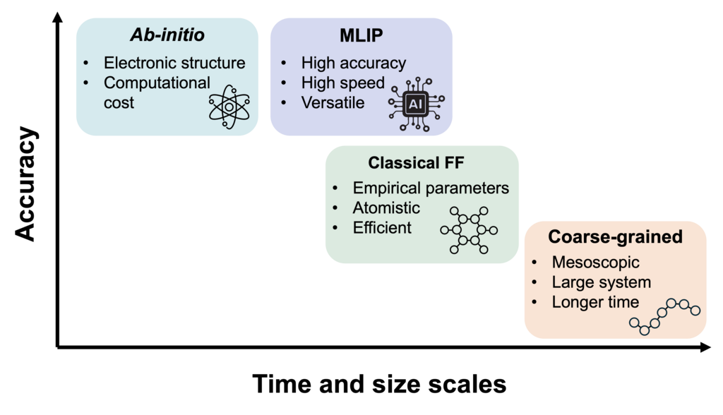
A key factor that determines the accuracy and applicability of MD simulations is the interatomic potential, or also called “force field". A force field is the foundation of any MD simulation, consisting of a set of potential functions (the mathematical equations describing interatomic interactions) and their corresponding parameters.

Selecting an appropriate force field that aligns with the system of interest and the goals of the study is essential for producing reliable and meaningful simulation results. In this section, we introduce the major categories of interatomic potentials commonly used in computational chemistry, highlighting their key characteristics, typical applications, and practical considerations for selecting the right one.

(1) Ab-initio Molecular Dynamics

Ab initio MD (AIMD), also known as first-principles molecular dynamics (FPMD), is a simulation method in which interatomic forces are calculated directly from the principles of quantum mechanics, without relying on empirical parameters.By explicitly solving the electronic structure, AIMD is particularly well suited for investigating phenomena where changes in the electronic state are critical, such as bond formation and breaking, chemical adsorption on surfaces, and catalytic reactions.

A major limitation of AIMD, however, is its high computational cost. Since quantum chemical calculations must be performed at every time step to determine the electronic structure, this approach is far more demanding than empirical or semi-empirical methods. As a result, the typical system size that can be simulated is limited to several hundred atoms, and the accessible timescale is usually on the order of picoseconds (10⁻¹² seconds).

(2) Classical Force Fields: An Atomistic Simulation

Classical force fields describe interatomic interactions using pre-defined potential functions and a set of parameters optimized for specific atom types. These parameters are carefully calibrated to reproduce experimental data or results from quantum chemistry calculations, allowing classical force fields to be applied across a wide range of materials and molecular systems.

For material science applications, the following force fields are frequently considered:

• Born-Mayer-Huggins (BMH) potential: for ionic crystals (e.g., alkali halides, silicates).
• Buckingham potential: for rare-gas crystals, molecular solids, oxides, and ceramics.
• Stillinger-Weber potential: for covalently bonded semiconductors (e.g., silicon, germanium).
• Embedded Atom Method (EAM):  for metallic and alloy systems.
• Tersoff: for strongly covalent materials (e.g., silicon, carbon).
• Dreiding:a general-purpose force field for a wide range of elements, primarily used for organic molecules.
• UFF(Universal Force Field): a general-purpose force field designed to cover a broad range of elements, both organic and inorganic.

For biomolecular systems, force fields specifically optimized to accurately reproduce the structure and properties of macromolecules such as proteins, nucleic acids, and lipids are commonly used. Widely used force fields include:

• AMBER (Assisted Model Building with Energy Refinement)
• CHARMM (Chemistry at Harvard Macromolecular Mechanics)

​

A major advantage of classical force fields is their computational efficiency. In particular, by leveraging GPUs, it is possible to conduct simulations for systems containing hundreds of thousands to millions of atoms, reaching timescales on the order of microseconds (μs).

(3) Coarse-Grained Force Fields: Simulating Mesoscopic Phenomena

Coarse-grained (CG) models significantly reduce computational cost by representing groups of atoms—such as an amino acid residue or a polymer monomer—as a single interaction site or particle. This simplification enables simulations of much larger systems and longer timescales, making it possible to explore mesoscopic phenomena such as the self-assembly and phase separation of polymeric materials, lipid membranes, and nanostructures.

Representative coarse-grained models are, for example,

• MARTINI:  for biomolecules (lipids, proteins), polymers, and surfactants.
• SPICA: for biomembranes, soft matter, and proteins.

While CG models are well-suited for investigating large-scale phenomena, it is important to recognize inherent trade-offs. By averaging out atomic-level details, these models generally lack the resolution needed to capture fine-grained features such as specific interatomic interactions (e.g., hydrogen bonds, salt bridges, π–π stacking), solvation effects, and chemical reactions. 

Moreover, applying CG models effectively requires careful consideration. Key challenges include choosing an appropriate level of coarse-graining, designing accurate interaction potentials, and parameterization tailored to the system under study. These steps are essential to ensure that the CG model faithfully represents the physical behavior of the system under investigation.

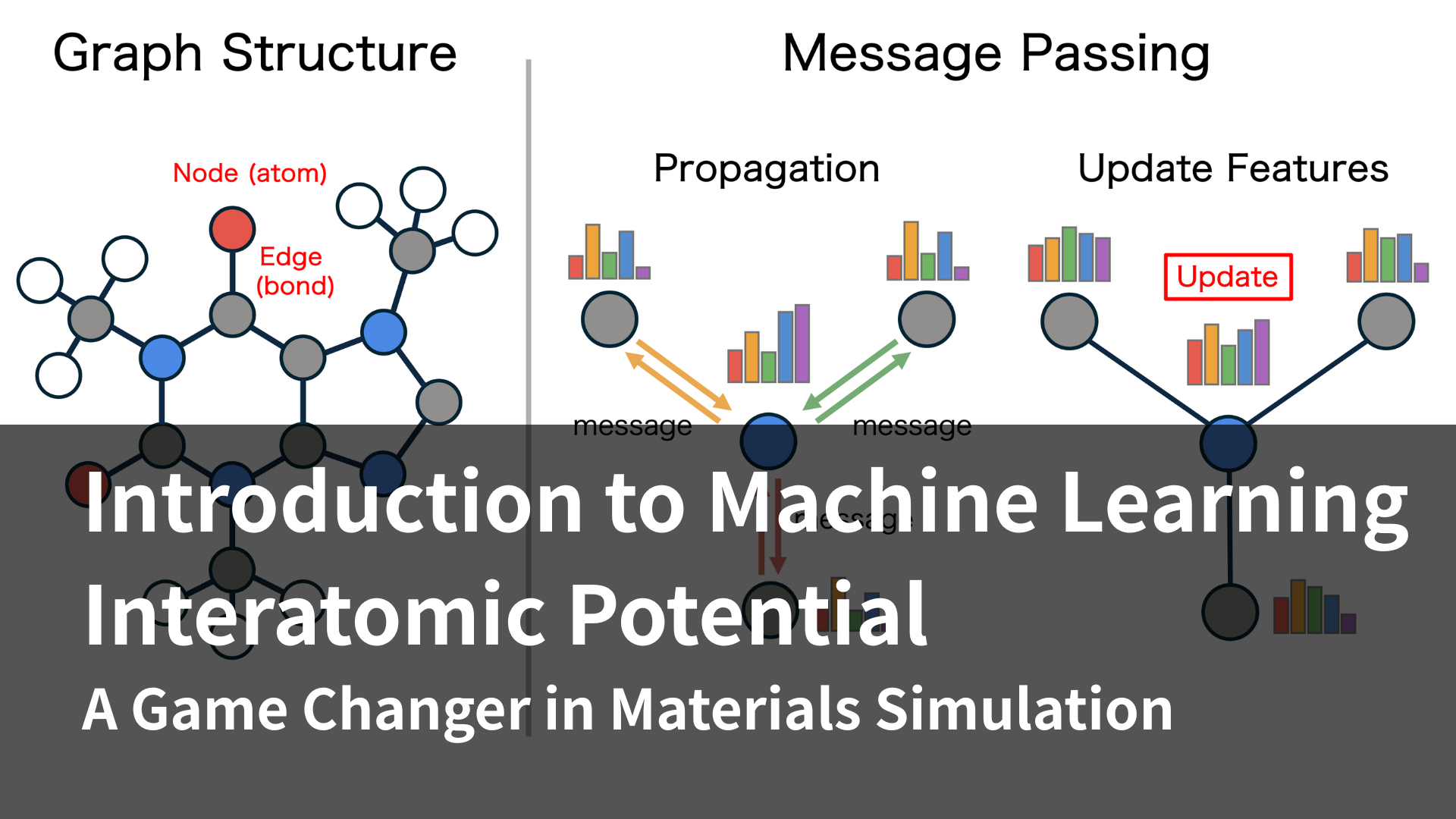
(4) Machine Learning Interatomic Potential: A Breakthrough balancing Accuracy and Speed

One of the most significant recent innovations in MD simulation is the “Machine Learning Interatomic Potentials” (MLIPs). This groundbreaking approach leverages AI technologies like neural networks to overcome the long-standing trade-off between accuracy and computational speed.

MLIPs are trained on large datasets derived from first-principles calculations, such as density functional theory (DFT). These datasets typically contain energies and atomic forces corresponding to a wide variety of atomic configurations. Neural network models learn the underlying patterns in this data, enabling them to reproduce interatomic forces with an accuracy comparable to quantum mechanical calculations.

Recent advances have also focused on developing universal MLIPs that cover a broad range of elements across the periodic table. A notable example is the Preferred Potential (PFP), which powers atomic-scale simulation platform, Matlantis.

Traditionally, conducting accurate simulations for new materials and molecules required extensive effort to identify or fine-tune a suitable force field, which is a time-consuming and labor-intensive task. In contrast, universal MLIPs like PFP eliminate the need for system-specific parameter optimization, allowing users to simulate diverse materials with no system-specific tuning. 

Another major advantage of MLIPs is their ability to maintain quantum-level accuracy while achieving remarkable computational speed. This makes it feasible to simulate large systems—on the order of tens of thousands of atoms—over extended timescales of tens of nanoseconds, which would be prohibitively expensive using conventional DFT methods. As a result, MLIPs are now being applied to a wide range of complex systems and phenomena, including:

• Amorphous materials and high-entropy alloys with disordered atomic structures
• Ionic transport and diffusion dynamics in solid electrolytes and liquid environments
• Reaction mechanism exploration on catalytic surfaces and in solution
• Interfacial behavior at boundaries between heterogeneous materials (e.g., alloys, ceramics, and organic compounds)

The emergence of MLIPs is transforming the landscape of molecular simulation, unlocking new possibilities in materials and molecular science and significantly accelerating materials and molecular discovery and innovation.

Summary

In this article, we introduced the fundamentals and applications of molecular dynamics simulations which is often described as a “computational microscope.” Beyond traditional approaches such as ab-initio, classical, and coarse-grained simulations, the recent emergence of machine learning interatomic potentials has significantly broadened the scope of MD simulations—effectively bridging the long-standing gap between accuracy and scalability.

As molecular dynamics simulations become more accessible and widely adopted to more researchers, the material and molecule research and development will undoubtedly accelerate. Molecular dynamics simulations are no longer just a tool for understanding physical phenomena—it is evolving into a powerful engine for innovation, enabling simulation-driven, rational design of new materials and molecules before any experiments.

Are you looking to accelerate your R&D with simulation? Matlantis, powered by a machine learning potential trained to cover the entire periodic table, was developed precisely to support this transformation. With Matlantis, you can instantly explore new ideas across a wide variety of materials the moment inspiration strikes. Molecular dynamics simulations stand as a core technology poised to lead the next generation of materials and molecule development.

References

[1] Statistical Mechanics: Theory and Molecular Simulation (M. E. Tuckerman)

[2] Understanting Molecular Simulaton From Algorithms to Applications (D. Frenkel & B. Smit)

[3] Computer Simulation of Liquid (M. Allen & D. J. Tildesley)