Explainer : Why Did the AI Predict That ? Uncovering Atomic-Level Interpretability through PFP Descriptors and Shapley Values

The online proceedings for the Spring Meeting of the Japan Society of Applied Physics have been released, signaling the arrival of academic conference season. Many people are busy preparing their presentations after submitting their proceedings, and many others are looking at the published proceedings and making plans to attend.

Last year, I gave a presentation at the 86th Autumn Meeting of the Japan Society of Applied Physics entitled " Atomic Level Explanation via PFP Descriptors and Shapley Values." I was fortunate to have a large audience that day, and it was very well received. It was an opportunity to get a firsthand feel for just how high the demand is for "explainability," or "why AI made the predictions it did" in the field of materials informatics (MI).

So, with the arrival of the academic conference season, I have written an article based on the content of the presentation at the time. I will provide a thorough explanation, including detailed background and prerequisite knowledge that could not be fully conveyed in the short time frame of the conference.

1. What are PFP descriptors?

First, we will explain PFP descriptors, which are used as machine learning descriptors. PFP descriptors are a function that outputs information from the final layer of the universal machine learning potential  (PFP) [1]. Each atom is assigned a 256-dimensional vector that represents its surrounding environment. While each of these 256 values does not have an intuitive physical meaning, they contain advanced information that supports the accuracy of PFP calculations. It has been reported that by repurposing this information, the physical properties of materials can be predicted with high accuracy [2, 3].

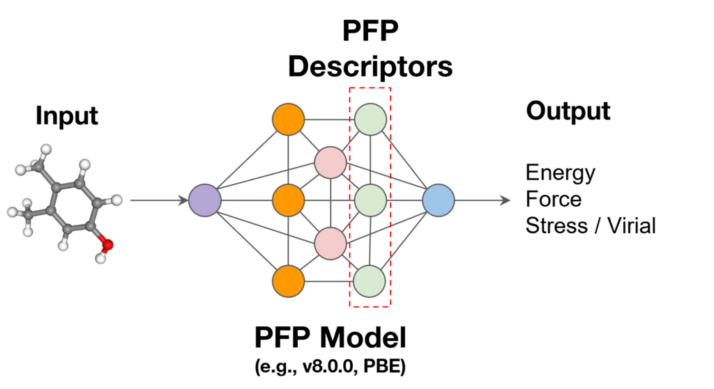
Figure 1. PFP descriptors

2. What is the Shapley value?

Next, we will introduce the Shapley value, which is central to explaining machine learning models. The Shapley value is a concept used in game theory, and is a calculation method for distributing the gains made by the entire team according to each player's contribution. The central idea is to consider all possible scenarios and determine the average value as that player's contribution.

2-1. Specific examples

Let's explain this using the following example. Suppose there are three players, A, B, and C, and the payoffs obtained from each combination of participation are defined as shown in Table 1. In this case, how should the payoff obtained from all three players' participation be distributed to each member?

Table 1. Relationship between players and payoffs

Participating players	gain
No one participates	0
A	1
B	2
C	3
A, B	6
A, C	7
B, C	8
A, B, C	15

Here, we consider a member's contribution based on "how much the gain increased by that player joining the team."

However, the amount of increased benefit depends on who is already on the team.

• If A joins a group where no one else is present (gain: 0) and A joins (gain: 1): A's contribution is 1
• If A joins a group where B already exists (benefit: 2) and A joins (benefit: 6), A's contribution is 4.

In this way, the amount of gain that is gained varies depending on the members already in the group. Therefore, we consider all patterns of members already in the group and average them to define the contribution of each member.

The specific calculation is shown in Table 2. For example, let's look at the case where participants are A → B → C.

• If A joins a group where no one else is present (gain: 0) and A joins (gain: 1): A's contribution is 1
• If A already exists (benefit: 1) and B joins (benefit: 6): B's contribution is 5
• If A and B are already there (gain: 6) and C joins (gain: 15): C's contribution is 9

The Shapley value for each member is calculated in this way for all patterns and averaged (the bottom row of Table 2). As can be seen from the calculation results, the Shapley value has a very favorable property for distribution: "the sum of each member's contribution equals the total payoff when all members participate."

Table 2. Contribution of each player

Participation order	A's contribution	B's contribution	C's contribution
A → B → C	1	5	9
A → C → B	1	8	6
B → A → C	4	2	9
B → C → A	7	2	6
C → A → B	4	8	3
C → B → A	7	5	3
average	4	5	6

2-2.Generalization and approximation methods

The above operation can be generalized to the following formula:

where Φ _i is the contribution of player i, N is the universe of players, S is the subset, | S | is the number of players in the subset, | N | is the total number of players, and ν is the value function used to calculate the payoff from participating players. The Shapley value has the good property that the sum of each player's contribution equals the payoff, but when the total number of players is n, the computational order is O(2 ⁿ), which is very high. Therefore, a method has been proposed to approximate the Shapley value using linear regression weighted by the following Shapley Kernel [4].

z' is a one-hot vector indicating whether each player is participating, and M is the total number of players. Please refer to the paper for proof that the Shapley Kernel can be used to approximate this. (The Python code to calculate this example using the Shapley Kernel is included in the appendix. Please make use of it.)

3.Explanation via PFP descriptors and Shapley values

So how do we combine these to explain material properties? And why do we use PFP descriptors? The reason is that PFP descriptors have significant advantages over ordinary material descriptors.

In conventional machine learning models, a specific feature cannot simply be excluded from the input, even if one does not wish to consider it.

However, PFP descriptors are "features for each atom." The features of each atom can be aggregated (readout) through calculations such as summation, and then converted into a descriptor for the entire molecule. Therefore, even if you ignore (mask) the features of a certain atom, the number of dimensions of the vector after readout remains unchanged, and you can input it directly into the model to calculate predicted values.

This makes it possible to artificially create "predicted values when a certain atom is not present" and calculate the Shapley value for each atom. In other words, it is possible to quantitatively show "how much each atom contributed to the predicted value."

Because PFP descriptors are latent variables of a model trained on a large amount of data in advance, it is possible to build a machine learning model that can predict material properties with high accuracy. When interpreting the predictions of a machine learning model, valid results cannot be obtained by interpreting a model with low predictive accuracy. Therefore, combining PFP descriptors with Shapley values is thought to make it easier to obtain chemically valid explanations.

Analysis example: Water solubility of 3,4-dimethylphenol

In fact, we constructed a machine learning model to predict the water solubility of organic molecules, and the results of interpreting the predicted water solubility of 3,4-dimethylphenol are shown in Figure 2.

Red indicates a positive contribution, blue a negative contribution, and the intensity of the color indicates the magnitude of the contribution. Methyl groups and benzene rings are blue, and hydroxyl groups are red, confirming that this is consistent with known chemical knowledge. When calculating the Shapley value, masking each functional group rather than each atom allows for interpretation at the functional group level.

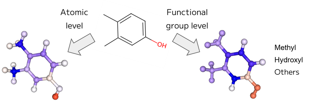
Figure 2. explanation of the predicted water solubility of 3,4-dimethylphenol

Example code for this method is available in the Matlantis environment, so please give it a try.

Supplement: What is different from the method used in the shap package? 

The shap package [5] approximates the absence of features by marginalization, but this has problems with computational cost and approximation error. Our method using PFP descriptors can directly mask each atom, eliminating the need for marginalization and reducing computational cost and error.

4.About this year's Spring Academic Conference of the Japan Society of Applied Physics

So far, I have introduced the contents of my presentations from last year. At this year's Spring Academic Conference of the Japan Society of Applied Physics, our company will be making the following four academic presentations.

This presentation will span different sessions covering phase diagrams, battery materials, semiconductor materials, and enzyme reactions. We hope that it will serve as an example demonstrating that the universal machine learning inter-atomic potential can be applied to a wide range of topics, from physics and materials to biology.

[List of our announcements]

Temperature Dependence of Ternary Phase Diagrams Using Universal Machine Learning Inter-atomic Potential

Hiroki Kotaka (Matlantis Corporation)

Analysis of Structural Stability and Irreversible Changes in Li-Ion Battery Cathode Materials Using uMLIP

Kota Matsumoto, Takahiro Hirai (Matlantis Corporation)

Prediction of Vapor Pressure Parameters Based on Adsorption Free Energy Calculations of ALD Precursors Using uMLIP

Yusuke Asano (Matlantis Corporation)

Enzymatic Reaction Mechanism and Free Energy Analysis using Universal Machine Learning Interatomic Potential

Yoshitaka Yamauchi (Matlantis Corporation)

In addition, this year our company representative, Okanohara, will be giving a lecture in the public section.

How the Evolution of Semiconductors Creates Intelligence

Daisuke Okanohara (Preferred Networks / Matlantis)

We look forward to discussing this with you all at the venue on the day!

Appendix: Example of Shapley Kernel calculation using Python

This is the Python code introduced in the main text that calculates the player's contribution using the Shapley Kernel. By running this, you can confirm that the Shapley Kernel can approximate the Shapley value.

import itertools
import math
import numpy as np

coalition_to_value = {
    (0, 0, 0): 0,
    (1, 0, 0): 1,  # A
    (0, 1, 0): 2,  # B
    (0, 0, 1): 3,  # C
    (1, 1, 0): 6,  # A, B
    (1, 0, 1): 7,  # A, C
    (0, 1, 1): 8,  # B, C
    (1, 1, 1): 15, # A, B, C
}

M = 3

coalitions_binary = list(itertools.product([0, 1], repeat=M))
X = np.array(coalitions_binary)

y = np.array([coalition_to_value[c] for c in coalitions_binary])

def shapley_kernel_weight(M, s):
    if s == 0 or s == M:
        return 1e9 
    else:
        combinations_term = math.comb(M, s)
        denominator = combinations_term * s * (M - s)
        kernel_weight = (M - 1) / denominator
        return kernel_weight

kernel_weights = np.array([shapley_kernel_weight(M, np.sum(c)) for c in coalitions_binary])

X_matrix = np.hstack((np.ones((X.shape[0], 1)), X))
    
sqrt_weights = np.sqrt(kernel_weights)
X_weighted = X_matrix * sqrt_weights[:, np.newaxis]
y_weighted = y * sqrt_weights

coeffs, _, _, _ = np.linalg.lstsq(X_weighted, y_weighted, rcond=None)

shapley_values = coeffs[1:]

print(f"{shapley_values=}")

References

[1] PFP Descriptors, (accessed January 30, 2026)

[2] Z. Mao et. al., npj Comput. Mater.  10, 265 (2024).

[3] The Power of PFP Descriptors: Enhancing Prediction Tasks with Pre-trained Neural Network Potentials, (accessed January 27, 2026)

[4] S. M. Lundberg, S. I. Lee., Adv. Neural Inf. Process. Syst. 30 (2017).

[5] https://github.com/shap/shap (accessed January 30, 2026)