In research and development, particularly in material development, challenges arise regarding the time and cost of experiments and securing human resources. In this context, simulation-based approaches using computational chemistry are receiving attention. Specifically, DFT (Density Functional Theory), which calculates electronic states based on quantum mechanics, offers a balance between computational cost and accuracy, and its application in research and development is expanding.
In this article, we will provide a clear explanation of representative software for performing DFT calculations, including selection criteria, compatible visualization tools, and the actual calculation process. Finally, we will briefly introduce a comparison with high-speed calculations using our product, “Matlantis”.
DFT Software Selection Guide
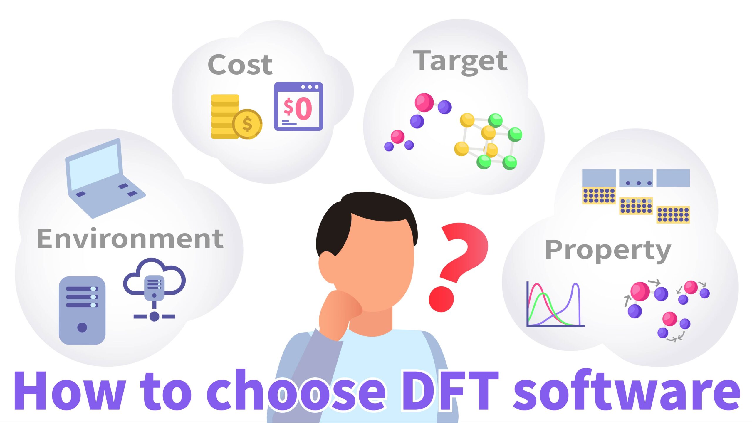
There are various types of software capable of performing DFT calculations, and it is essential to select the appropriate software to achieve the desired computational results. This guide provides an overview of the fundamental considerations for selecting DFT software, including the target materials, desired physical properties, computational environment, and budget.
Target material system
The choice of standard computational methods in DFT calculations depends heavily on the specific material system under investigation. Therefore, it is necessary to determine in advance whether your target material is a "solid system" or a "molecular system". These can be roughly classified as follows.
“Solid systems” include solids such as metals and semiconductors, as well as amorphous materials and solutions with aggregated structures. Assuming the input structure is periodically repeated (periodic boundary conditions) makes calculations for infinitely large systems possible. If you want to calculate the electronic states or physical properties of a collection of atoms or molecules, select DFT software designed for solid systems.
“Molecular systems” refer to molecules such as water (H₂O) or methane (CH₄), as well as molecular clusters formed by their interactions. Although these systems are typically treated in a vacuum, calculations considering solvent effects are also possible. For applications such as calculating the properties of individual molecules or the reactions of homogeneous systems with high precision, molecular system-oriented DFT software is more suitable.
Target physical properties and phenomena
Then, you need to figure out the specific properties you want to calculate. In general, any property related to electronic states can be evaluated through DFT calculations.
It is vital to compare calculated properties with experimental data to ensure their validity. Given that different software packages support varying sets of properties, it is crucial to verify beforehand if your chosen software is compatible with the experimental data you have available.
The table below lists common characteristics and phenomena that can be addressed by DFT calculations, along with representative examples of the results obtained.
| Characteristic/Phenomenon for Calculation | Example of calculation results |
| Structural Properties | Lattice constant, Surface structure, Equilibrium geometry, Volume, Density |
| Electronic Properties | Band structure, Density of states, Molecular orbitals, Partial Charge, Dipole moment |
| Thermodynamic Properties | Specific heat, Heat capacity, Boiling point, Melting point, Formation energy, Surface energy, Free energy |
| Transport Properties | Electrical conductivity, Diffusion coefficient, Thermal conductivity, Viscosity |
| Response functions and optical properties | Elastic constants, Dielectric constant, Magnetic moment, Phonons, Molecular vibrations, UV-VIS absorption wavelength and intensity |
| Chemical Reactions | Reaction energy, Activation energy |
While in theory, DFT can address many experimental properties linked to electronic states, it's important to recognize that practical application might be limited for certain time and spatial scales. Realistically, the upper bounds for time and spatial scales accessible via DFT calculations are typically on the order of nanoseconds and nanometers, respectively.
Viewer Options
Performing DFT calculations necessitates three-dimensional coordinates of the target system as input. While structures can sometimes be sourced from public databases or existing literature, structural modeling becomes essential if they are not readily available. Furthermore, DFT calculation outputs are typically presented in numerical, text-based formats. Depending on the complexity of the calculation, these outputs can be tens of thousands of lines long. This makes it hard, especially for beginners, to find the relevant information.
To address this problem, "viewers", which are visualization software, are widely employed. Many viewers also incorporate structure modeling functionalities, commonly used for constructing complex molecules or surface adsorption systems. Official viewers, when compatible with the DFT software, can directly retrieve and display information such as energy and charge from the output files. These tools are particularly effective for visualizing data like structures, molecular orbitals, and vibrations, which are hard to interpret from raw numerical data alone.
A variety of viewers exist, and it is crucial to select one that is compatible with your chosen DFT software. Viewers differ in their visualization capabilities, features, usability, support systems, and pricing (paid or free), making it important to review these aspects prior to implementation.
Available Environments and Resources
Before undertaking DFT calculations, it is critical to assess your available computational resources, including your computer hardware and overall computing environment. While calculations of smaller target systems can be performed on standard personal computers, dedicated computing machines are generally preferred for more extensive operations.
However, acquiring a new dedicated computing machine involves substantial upfront costs, the need for physical space, environmental considerations like power and cooling, and the requirement for specialized expertise and personnel for system setup and maintenance.
Moreover, calculations involving a large number of atoms (electrons) or those requiring high precision can significantly increase the computational load, with single calculations potentially taking several weeks. Consequently, limitations in computational resources often restrict the number of trials, posing a significant hurdle in research and development.
In recent years, alternative solutions have emerged to address computational resource constraints, including cloud services for computational environments and AI-driven technologies to accelerate calculations. For example, our cloud-based service, “Matlantis”, eliminates the need for infrastructure setup and utilizes machine learning for high-speed calculations, making it a valuable solution adopted in many research groups.
Budget and License
When choosing DFT software, it is important to consider both the initial cost and the license.
Software options typically include open-source (free) and commercial (paid) versions. Free software may have limitations in features, support, and licensing terms. For commercial software, academic licenses generally range from several hundreds to thousands dollars, while industrial licenses can cost ten times more or even higher.
There are different license options, including "named licenses" for individual users, "node-locked" licenses restricted to specific devices, and "site licenses" for multiple users within an organization. The specific conditions depend on the software. Another option is to use "contract calculation services." These services allow you to outsource calculations as needed without purchasing the software.
Comparison of Leading DFT Software
A summary of major DFT software is provided below. We have briefly outlined the main target system, features, compatible viewers, and license (paid or free) for each. For comprehensive specifications and the latest information, please consult the official websites of the respective software developers. To ensure a smooth implementation, it is also advisable to confirm initial setup and analysis support systems in advance.
| Software | Main Target System | Main Features | Main Compatible Viewer | License |
| VASP | Solid | Industry standard for solid-state/periodic system calculations |
p4vasp VESTA | Paid |
| Quantum Espresso | Solid | Free solid-state/periodic system calculation software | VESTA | Free |
| SIESTA | Solid | Electron mathematical representation can be adjusted to suit the purpose | VESTA | Free |
| Gaussian | Molecular | Industry standard for molecular system calculations, GUI version available |
GaussView Avogadro | Paid |
| GAMESS | Molecular | Free, active feature development |
MacMolPlt Avogadro | Free |
| ORCA | Molecular | Strong in optical properties and high-precision calculations |
Avogadro ChimeraX Chemcraft | Paid (Academic free) |
・For Solid Systems
Software options for solid-state systems include VASP, Quantum Espresso, and SIESTA. VASP is a commercial software widely recognized as the standard for solid-state calculations. Quantum Espresso and SIESTA are free and primarily used in academic environments. Compatible viewers include VESTA and p4vasp. Structures from calculation results can also be visualized using crystal structure software after conversion to CIF (Crystallographic Information File) or XYZ file formats (a simple format containing only atom count, element type, and 3D coordinates).
・For Molecular Systems
For molecular systems, available software includes Gaussian, GAMESS, and ORCA. Gaussian is a commercial software considered the standard for molecular calculations. GAMESS is a free software with ongoing active feature development. ORCA is a commercial software that offers a free version for academic users. Compatible viewers include GaussView (paid), Avogadro, and Chemcraft.
DFT Calculation Libraries for Python
For those considering a preparation of new dedicated computing environment for themselves, it typically involves command-line operations and compilation (transforming programs into machine-executable forms) within a Linux environment. Readers unfamiliar with these procedures may face hurdles during environment setup, potentially leading to additional costs.
To simplify this, Python libraries (collections of pre-developed programs) are available for DFT calculations, with PySCF and Psi4 being prime examples. Python is also extensively used in machine learning, and many readers probably already use it in their work. The ability to create structures and set calculation conditions using Python code makes these libraries an accessible option for Python users to get started with DFT calculations.
By integrating various Python libraries, it becomes possible to seamlessly manage the entire workflow, from acquiring computational data for material properties to conducting machine learning and data analysis. This synergy makes Python an exceptionally suitable environment for implementing Materials Informatics (MI), a field that has garnered significant attention recently.
Practical Steps to Start DFT Calculations
Following the discussion on DFT software selection and the features of major tools, this section outlines the practical steps for executing DFT calculations. While specific procedures may vary by software, this general workflow serves as a useful guide.
Step 1: Set Up the Computing Environment
Begin by installing the chosen DFT software and viewer on your personal computer or dedicated computing machine, strictly following the official manuals.
A larger number of CPU cores enables greater parallelization, which significantly enhances calculation speed. Dedicated computing machines often feature CPUs with tens to hundreds of cores. Additionally, incorporating GPUs can further accelerate calculations.
For larger calculations, such as those involving dozens or more atoms, requiring substantial computational resources, a more powerful computing environment is necessary. Cloud-based environments for executing DFT calculations also present a viable option.
Step 2: Create the Input File
Before performing DFT calculations, you must create an "input file" first. This is a text file that contains details about the target system and the computational method. DFT softwares perform calculations according to the contents of this file.
Specifically, the input file includes information about the calculation target, such as its 3D structure (atomic positions), total charge, and spin, along with the properties to be determined (e.g., energy, equilibrium geometry, vibration) and calculation parameters (e.g., functional, basis set).
Input files can be written directly in text format or generated via the graphical user interface (GUI) of viewers or modeling software.
Below is an example of an input file for geometry optimization of aspirin using GAMESS. The 3D structure of aspirin was retrieved from the public database PubChem (https://pubchem.ncbi.nlm.nih.gov/). This specific input was generated using a feature within the Avogadro2 viewer (https://www.openchemistry.org/projects/avogadro2/)
! Aspirin opt
$BASIS GBASIS=N31 NGAUSS=6 NDFUNC=1 $END
$CONTRL SCFTYP=RHF RUNTYP=OPTIMIZE ICHARG=0 MULT=1 DFTTYP=WB97X-D $END
$STATPT OPTTOL=0.0001 NSTEP=100 $END
$SYSTEM MWORDS=2 $END
$DATA
Aspirin
C1
O     8.0   1.23330   0.55400   0.77920
O     8.0  -0.69520  -2.71480  -0.75020
O     8.0   0.79580  -2.18430   0.86850
O     8.0   1.78130   0.81050  -1.48210
C     6.0  -0.08570   0.60880   0.44030
C     6.0  -0.79270  -0.55150   0.12440
C     6.0  -0.72880   1.84640   0.41330
C     6.0  -2.14260  -0.47410  -0.21840
C     6.0  -2.07870   1.92380   0.07060
C     6.0  -2.78550   0.76360  -0.24530
C     6.0  -0.14090  -1.85360   0.14770
C     6.0   2.10940   0.67150  -0.31130
C     6.0   3.53050   0.59960   0.16350
H     1.0  -0.18510   2.75450   0.65930
H     1.0  -2.72470  -1.36050  -0.45640
H     1.0  -2.57970   2.88720   0.05060
H     1.0  -3.83740   0.82380  -0.50900
H     1.0   3.72900   1.41840   0.85930
H     1.0   4.20450   0.69690  -0.69240
H     1.0   3.71050  -0.36590   0.64260
H     1.0  -0.25550  -3.59160  -0.73370
$END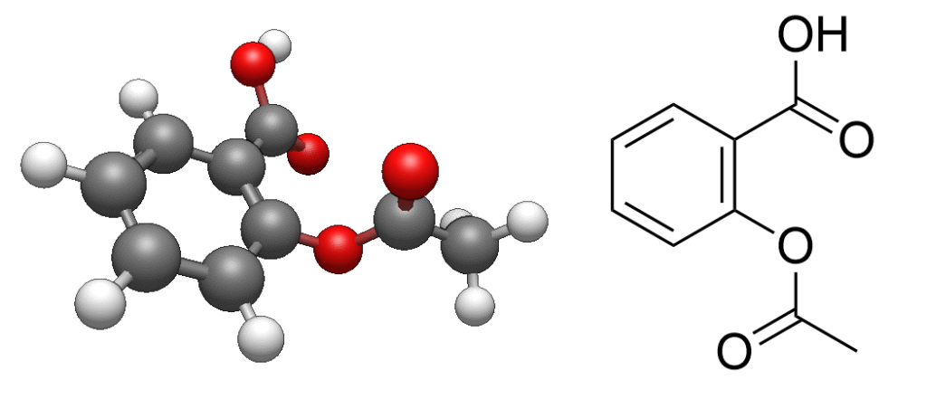
Step 3: Execute the Calculation and Review Output Results
Upon execution of a DFT calculation, the results are saved as an "output file", typically in a numerical, text-based format.
For example, when performing geometry optimization of aspirin using the input file created in the Step 2, the atomic positions progressively shift, eventually converging to a stable, lower-energy structure. The structure and energy at each stage of this process are recorded in the output file.
These output results can be visualized using the aforementioned viewer, greatly simplifying analysis. Loading the GAMESS output file into Avogadro2 will display the optimized structure, as shown below.
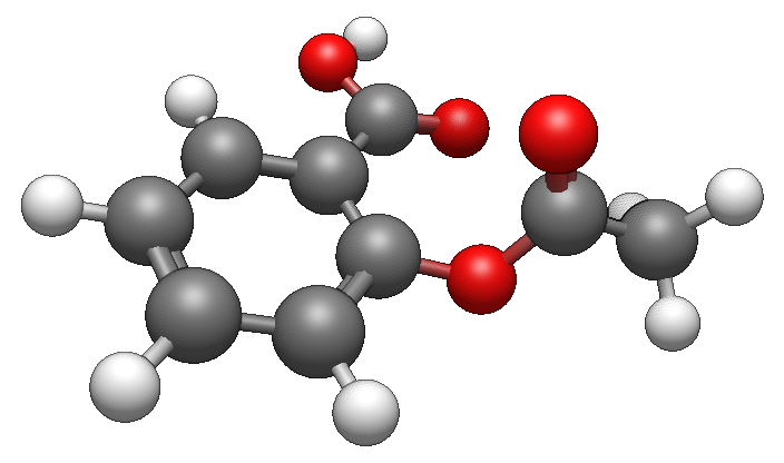
The geometry optimization reveals that the carboxyl group (-COOH) in particular has rotated to align with the aromatic ring. This demonstrates how such calculations provide insights into the molecule's 3D structure, which is not apparent from its chemical formula alone. Typically, molecules exist in their most stable conformation, so DFT calculations generally begin with structural optimization, followed by discussions of electronic states and properties based on the resulting stable structure.
This calculation took -6,400 seconds when run on a standard laptop (11th Gen Intel(R) Core(TM) i7-1165G7 @ 2.80GHz). When the same calculation was performed in parallel using multiple CPUs, it took -4,300 sec./2 cores and 3,900 sec./4 cores.
Comparison with Matlantis Calculations
Our product, Matlantis, offers a machine learning model capable of reproducing the results of the same DFT calculations (functional and basis set) as presented in the example above. When the same geometry optimization calculation was performed using Matlantis, it completed in approximately -9 seconds. Due to differing computational conditions, a direct comparison is not feasible, but this should provide a good sense of Matlantis's calculation speed.
In typical DFT calculations, the computational cost scales with the cube of the number of electrons in the system, meaning the speed difference becomes increasingly pronounced as the number of atoms grows. Matlantis can perform DFT-equivalent calculations -100,000 times faster for a 256 atoms system, and up to 2,000,000 times faster for a 3000 atoms system (refer to the "Product" section on our website for detailed information). This remarkable acceleration opens up possibilities for handling atom counts previously unfeasible with conventional DFT and enables high-throughput calculations for Materials Informatics (MI), addressing time-consuming challenges in these domains.
Furthermore, as Matlantis is a cloud service, users are freed from the burdens of environment setup and maintenance. Its design facilitates workflow within "Jupyter Notebook," a web browser-based application, leveraging various Python codes and libraries. This allows for the complete execution of tasks, including structure creation, visualization, analysis, machine learning, and the calculations themselves, all within the Matlantis environment.
Summary
This article has covered the selection process for DFT software, compared key options, and detailed the steps for implementation.
Given the diverse range of DFT software available, it is important to select the optimal solution based on your specific application, research objectives, budget, and operational framework. Moreover, establishing an appropriate computational environment is essential. Enhancing calculation speed allows for a greater number of trials, which directly translates to accelerated and more precise research and development. We sincerely hope this article assists you in choosing and implementing the DFT software that best suits your needs, thereby fostering advancements in your research and development efforts through DFT calculations. Matlantis, developed by our company, is a high-speed, general-purpose atomic simulation tool powered by machine learning. Accessible via a cloud environment, it delivers performance several orders of magnitude faster than traditional DFT methods. For those interested, we encourage you to explore Matlantis's calculation examples and introductory materials.
-


 URL
URL
Copied
Latest Articles
NEW
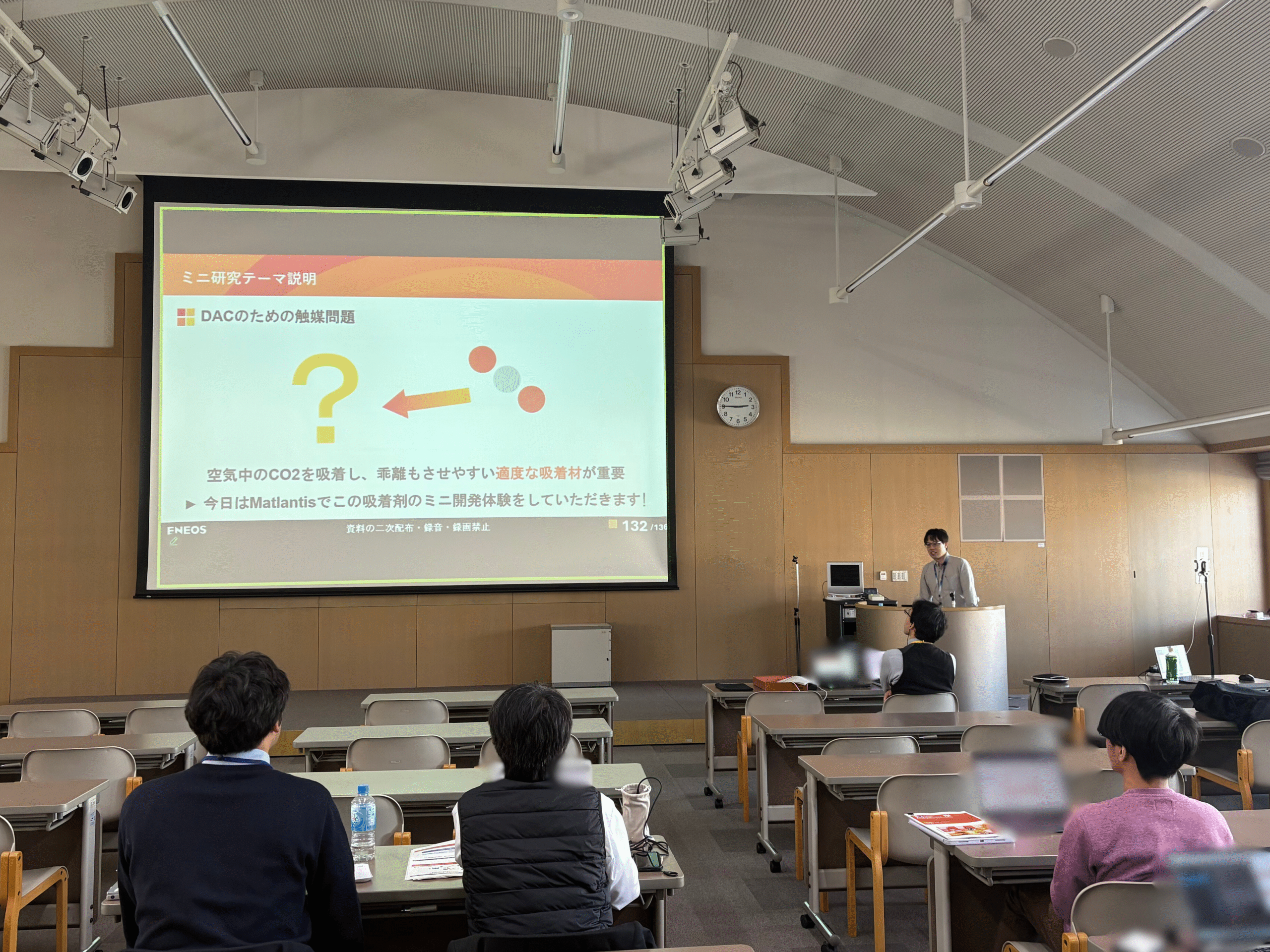
Learning AI materials simulation to accelerate research at the Fukui Kenichi Memorial Research Center, Kyoto University - Working with ENEOS to design the "best CO2 adsorbent"
NEW
Explainer : Why Did the AI Predict That ? Uncovering Atomic-Level Interpretability through PFP Descriptors and Shapley Values

Materials Informatics Explainer computational chemistry

Writing SMILES from scratch
Explainer computational chemistry

Nagoya University × Matlantis Case Study:“Advanced Experiments for Frontier Technologies and Sciences” —A Four-Day Intensive Course That Sparked Experimental Students’ Curiosity Through AI Simulation
Interview computational chemistry
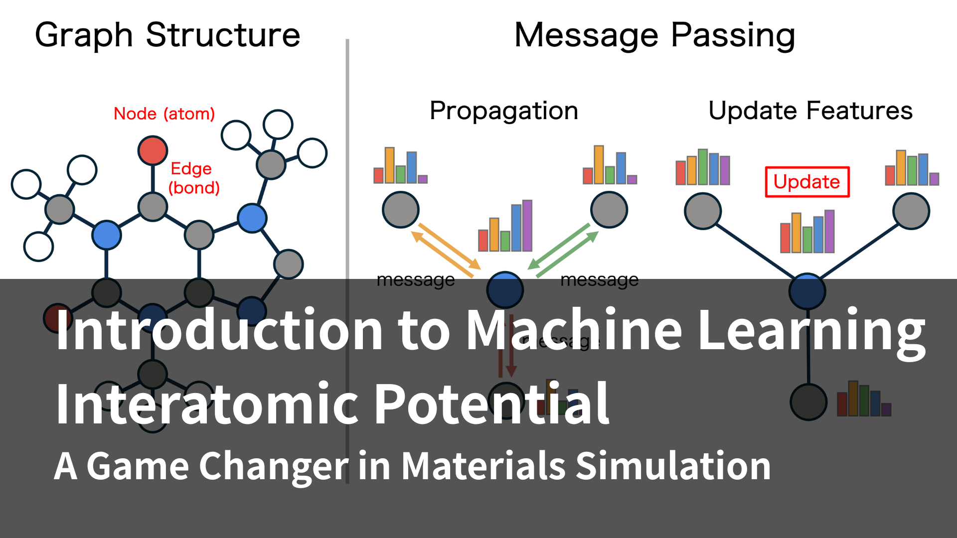
Introduction to Machine Learning Interatomic Potentials (MLIPs): A Game Changer in Materials Simulation

Machine Learning Interatomic Potentials Explainer