The Lab Is (Not) All You Need: Why autonomous laboratories make atomistic simulation more valuable, not less

1. The lab is speeding up

Picture a laboratory at 3 am where the lights are on, but no one is there. A robotic arm lifts a crucible from a furnace and carries it to an X-ray diffractometer. Software reads the diffraction pattern, decides the run missed its target, adjusts the recipe, and queues the next attempt. By morning, the system has worked through more experimental iterations than a graduate student completes in a month, minus the coffee breaks and occasional existential crisis. This is an autonomous laboratory, or self-driving lab: a system that plans experiments, runs them, reads the results, and decides what to try next, closing the loop with little or no human involvement.

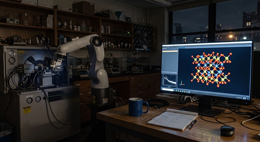
When I was a postdoc, such dreams lived only on the last slide in somebody's keynote (the one about where the field might go someday), but now they routinely appear as methods sections in Nature or Science papers.

As these approaches have matured, the funding has followed. In July 2026 the U.S. National Science Foundation put $400 million into a national network of AI-programmable cloud laboratories, remotely accessible facilities that researchers anywhere can drive with their own workflows. (In fact, Matlantis is a partner in one of them). The Department of Energy also announced $293 million for its Genesis Mission (with total federal commitments at nearly $5 billion), and the first project list is full of digital twins and closed loops. Private capital is flowing the same way, with advanced materials startups raising sums that make a federal grant look like a rounding error.

The clear goal is for autonomous experimentation to become ordinary research infrastructure.

2. The question for simulation

When experiments run this fast, there is a fair question that follows, and I have gotten it many times over the past year.

If a robot can synthesize and test hundreds of candidates this week, why simulate anything at all?

After all, if experiments are the "ground truth," why don't we just run a bunch of them?

That is a completely reasonable argument, and the counter to it has nothing to do with brute force since nobody is proposing to run a million experiments. In a self-driving lab, Bayesian optimization over composition and process variables will find an optimum in a small fraction of the samples a grid search would need, which is the whole point of putting a decision algorithm on top of a robot. (By the way, if you would like a primer on how these systems work, covering the robotics, the Bayesian decision-making, and the closed loop, see our earlier explainer on lab automation .)

As a simulation vendor, our honest answer is that experimental throughput and computational insight do different jobs, and speeding one up increases the value of the other.

The reason comes down to how the two sides scale. Experimental throughput grows linearly (i.e., you double the robots and you double the samples per week). However, the search space does not play along. Add one more element or one more processing variable and the candidate count explodes combinatorially. So the faster the lab runs, the more it costs to point that speed at the wrong region, and the more you want something that tells you where not to bother looking. That something is atomistic simulations. But the traffic runs both ways, too (more on that later).

Basically, atomistic simulations are not just "nice to have," but actually play an integral part in the discovery loop itself. Here I want to show why, and then describe how tightly these two halves can actually be connected.

3. The established division of labor

Thus far, simulation and experiment have generally worked together in two ways.

Role 1: Narrowing the field before the robot starts

Let's start with the most familiar arrangement, because the math is hard to argue against. You take a defined problem, set up a modest multicomponent design space, a few elements with a range of compositions and a handful of processing variables, and end up with millions of candidates. Even at a heroic 100 samples per day, exhaustively testing that space experimentally would take decades. You would finish the campaign, publish, and retire, in roughly that order. The funnel above the robot has to be computational.

Some of the most successful campaigns of the past few years are built exactly that way. In a collaboration between Microsoft and Pacific Northwest National Laboratory, 32 million candidate battery materials were screened down to roughly two dozen in about 80 hours of computation, one of which was then synthesized into a working solid-state battery prototype.

The same pattern sits underneath Berkeley Lab's A-Lab, whose synthesis targets were drawn from a computational screen of predicted-stable compounds; over 17 days of continuous operation it went on to make dozens of them [1].

However, it is worth being careful about what a screen like that actually delivers. One cannot directly compute "is this a good catalyst" or "is this a good battery" under all possible operational conditions. Instead, one computes a proxy: an adsorption energy, a diffusion barrier, a formation energy, a distance above the convex hull. The proxy stands in for the macroscopic observable(s) you care about, and how well it stands in can vary enormously from one problem to the next.

Meta's Open Catalyst Experiments 2024 (OCx24) effort is a clear public demonstration of both halves of that. The team paired an experimental campaign of 572 synthesized catalyst samples with a computational one, calculating adsorption energies for six reaction intermediates across roughly 20,000 materials by performing 685 million machine learning-accelerated relaxations[2]. For the hydrogen evolution reaction, the computational screen essentially recovered the classic activity relationship and placed platinum at the apex, which is notable because there was no platinum in the model's training data. However, for the CO2 reduction reaction, the computed descriptors were much weaker predictors of what the catalysts actually did in the cell, because selectivity there depends on far more than how strongly a single intermediate binds.

That is not an argument against screening, but rather an argument for knowing what screening is for. A computational funnel is extremely good at removing candidates that cannot possibly work, which is most of them, but less reliable at ranking the top-most survivors. Computation makes the space small enough to walk through, and the lab decides what is actually true. This is also why a better search strategy alone does not close the question.

Role 2: Seeing what no instrument sees

The second job has nothing to do with screening, and if you run a lab, automated or not, it may be the one you use more often.

An autonomous lab can tell you that a synthesis failed but does not tell you why. Was the target phase outcompeted by a more stable byproduct? Did an intermediate form and then decompose? While the diffraction pattern records the outcome, the mechanism happened at the atomic scale and disappeared, out of sight of instruments in the room. These are not just my random musings.

Take a look at the aforementioned A-Lab. When the team analyzed unsuccessful syntheses using computed reaction driving forces, many failures pointed to direct, actionable improvements in how targets are screened and recipes are designed [1]. And it is not only the failures that make the point. When A-Lab's reported results were later audited, 36 of the 40 compounds held up, but four could not be confirmed from the X-ray data alone and one had already appeared in the training set. The robot had done its part; what a diffraction pattern cannot do by itself is settle what was actually made, and that adjudication is exactly where a physical model earns its place. 

Simulation also offers something no physical experiment can, which is the ability to construct perfectly-controlled counterfactuals. That is, change a single variable (e.g., insert a single defect, swap a single dopant, change the surface termination), hold everything else fixed, and simulate. Experiments produce surprises that nobody plans for, and weeks can pass trying to explain them. In practice this makes simulation a "debugger." For example:

1.  You get an XRD pattern with a peak that should not be there. So you compute the formation energies of plausible competing and metastable phases, and the culprit turns up in an afternoon.
2.  A property that was stable for ten batches suddenly drifts in your new sample. A series of defect and impurity calculations reveal which contaminant could plausibly cause the change.
3. A film that deposits beautifully on one substrate refuses to nucleate on another. Precursor decomposition pathways and surface reaction barriers explain what the process window is really sensitive to.

If you want to see what this kind of analysis actually looks like in practice, we have written up a case study on methanol synthesis catalysts [3]. Computed IR spectra of intermediates were matched against in-situ DRIFT to determine what was actually on the surface, and that same structural picture then drove a dopant screen for stability and activity that was confirmed in the lab, where the chosen rare-earth-doped catalysts raised methanol yield by up to 28% at 360 °C while suppressing the CO side reaction. The lesson buried here is that, again (cf. OCx24 above), a single idealized slab could not reproduce the spectrum or separate active from inactive dopants, but a spread of realistic surface structures, combined, could. 

Such fast, physics-grounded checks belong inside these loops, not only in post-hoc analysis.

4. How tightly can simulations and experiments be coupled? Five rungs

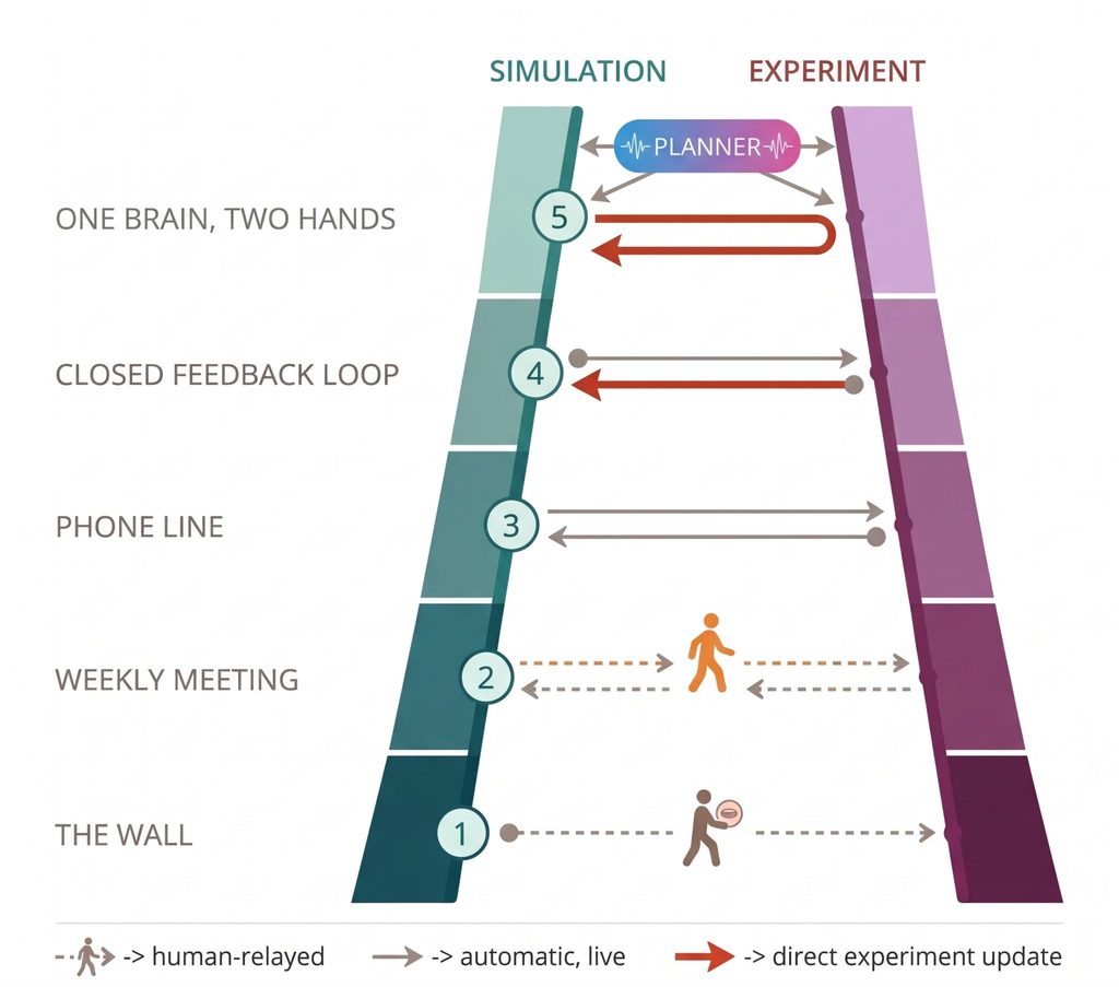
Everything I described above runs in one direction, with simulation informing experiment. At a recent event, however, we were actually asked an interesting question: can the traffic run both ways? Can experimental results make the simulations better? I believe they can. However, "simulation and experiment working together" covers an enormous range of arrangements, so it helps to divide these into rungs.

Rung 1, the wall. Simulation runs first, hands something over, and never hears back. If the lab discovers that your top candidate cannot be made at any temperature a furnace can reach, the screen never finds out, and you will cheerfully rank it first again next quarter.

Rung 2, the weekly meeting.  The two sides take turns, with humans carrying results between them. The computational team screens, the lab tests, and everyone gathers on Thursday to find out what the other half has been doing since last time. I have sat in many of these meetings and while they are genuinely useful, they are also why a promising result can languish in somebody's slide deck for six days before anyone acts on it.

Rung 3, the phone line. When I was a kid, a phone line was a thing you used to talk to people, live, while they talked back (n.b., although my last name is Young, I am, much to my chagrin, getting older every year). You asked a question, you got an answer, you adjusted. Here the campaign itself places the call mid-run, without a human in the middle, because the planner wants to know what the calculation says before it commits the robot to a composition.

Rung 4, the feedback loop.Now the direction of learning reverses, and experimental results start improving the computational model while the campaign runs. The model you finish with is not the model you started with, and the difference came from the lab.

Rung 5, one brain and two hands. Now the two feed each other. Experiments retrain the model so its next prediction is sharper, and the sharper model narrows what the lab bothers to test, each pass making the other better. A single planner sits on top of this, treating "run an experiment" and "run a simulation" as two actions competing for one budget and choosing whichever buys down the most uncertainty per hour and per dollar. Experiments are slow, expensive, and authoritative while simulations are fast, cheap, and approximate. The planner therefore spends each where it pays off the most. 

4a. So where is everybody?

Real campaigns do not sort cleanly onto a single rung, and the interesting ones sit across several. So rather than forcing each one into a rung, here is a more general overview of what the literature looks like.

Many recent excellent works sit near the first couple of rungs, and demonstrate what computation is carrying. 

For example, in a 2026 collaboration between the University of Toronto and Kyushu University, excited-state DFT calculations narrowed a virtual library of 252 candidate laser molecules down to 51, and a self-driving lab then synthesized and optically characterized every one, turning up a near-infrared emitter past 700 nm that nobody had reported[4].

One protocol coming from RoboChem is an interesting yet more subtle case. When its optimizer had to choose among seven palladium precatalysts, what told it which ones resembled each other was a set of descriptors computed by DFT from a published ligand library, which is also what let the team switch substrates later and converge in four more experiments [5].

There are also works sitting further up the ladder. 

For example, the same Berkeley group behind A-Lab built an autonomous system for solid-state synthesis that computes thermodynamic driving forces for candidate precursor combinations mid-campaign, picking the set most likely to reach the target phase and revising when an attempt fails [6].

AMASE goes further, remapping a Sn-Bi thin-film phase diagram in one unattended run on 66 measurements where a grid search would need 400, by feeding each diffraction result back into CALPHAD, which refits its parameters and chooses the next temperature to sample [7].

Another study from Argonne did the same thing a level deeper, retraining an actual machine learning interatomic potential (MLIP) for hafnium oxide from diffraction data rather than refitting a thermodynamic model [8].

Finally, a recent study applies such thinking to thin-film growth, performing autonomous AFM measurements over a CrTaWV-Mo composition spread and feeding each roughness measurement back into a kinetic Monte Carlo model that retunes its bond energies until it matches the film, turning a generic growth model into one specific to that alloy [9].  As stated by the authors, the kMC model "progressively evolves into a material-specific 'digital twin'" as it updates its parameters from the measurements. 

As we can see, the makings of a rung 5 system are already here, at least on the experimental side. Atomistic simulations are here as a general participant and can be tuned by experiments, but agentic frameworks that plan and run these are actually here too, constituting the other half of a rung 5 system; I will come to those shortly.

5. How atomistic simulation can live in the loop, and what Matlantis is doing about it

Every experimentalist who has been handed a ranked list of predictions has a story about how the top candidate actually performed (i.e., it didn't and went to the garbage). That gap is real, but in industrial practice it is often not even about accuracy at all. Rather, the simulation describes a hundred atoms for a nanosecond while the product is microns across and has to last ten years. Frequently the calculation is not wrong at all, in that it answers its own question perfectly well. What actually has to change for physics to sit inside a running campaign is speed, reach, and who is allowed to drive.

5a. Speed and scale

A calculation that takes three weeks is a post-mortem tool rather than a collaborator, and it is already well known that conventional quantum mechanical calculations cannot keep pace with a robot. Machine learning interatomic potentials changed that, and universal potentials went further by removing the per-system model-development step, which matters in a loop because a campaign asks unanticipated questions and you cannot pre-train a bespoke model for a question you do not yet know is coming.

On the other hand, scale matters as much as speed. Where DFT is effectively confined to a few hundred atoms over picoseconds, MLIPs reach much further in length and time. That reach is also how atomistic physics gets anywhere near the scale where a product lives. And pairing an MLIP with coarse graining methods, microkinetics, kinetic Monte Carlo, phase field modeling, and the like, pushes that reach further still.

Matlantis PFP, our universal MLIP, reaches accuracy approaching its DFT reference across 96 elements with no per-material model development[10], and our proprietary inference system, PFVM, is what makes it fast enough to sit in a loop rather than a queue[11]. PFP reaches further than people tend to expect, as in a recent all-atom study of the PET-hydrolysis reaction in a whole PETase enzyme in water [12]. I will also note that this is not only our own assessment. On MLIP Arena, a third-party benchmark that grades potentials on physical soundness and real-world behavior rather than error against a fixed DFT reference, the latest PFP ties MACE-MPA for the top overall position and places first in three of the individual tasks (more than any other potential) [13].

Finally, PFP can be extended in a few directions. Pairing it with established engines like OpenMM opens up larger systems, which is what made calculating interfacial thermal resistance at a metal and polymer interface tractable [14]. And PFP Descriptors exposes the feature vectors the model builds internally, so you can map a search space nobody has catalogued, or feed those features into a model alongside your own measurements, XRD, spectra, images, so that simulation and experiment train one predictor together[15].

5b. Access

Speed does not remove the second barrier, which is that simulation helps nobody if using it requires the fluency of a computational specialist. Much of the wall between experimentalists and computation was made of skills. Beyond just applying the methodology, running a simulation requires careful scoping of the problem, preparing structure files, setting conditions and tuning parameters, benchmarking, and aggregating results.

Recently agents have been taking that wall down. For example, QUASAR, a three-agent system, spans DFT, MLIPs, MD, and Monte Carlo, trades cost against accuracy on request, and reproduced a published photocatalyst screening with no human guidance [16]. As another example, a recent Argonne system coordinates eleven agents from structure generation through analysis, with failure recovery built in [17]. The user hands an administrator agent a plain-language prompt and it farms the work out to LAMMPS specialists that build the structure, dig up a suitable interatomic potential, write and submit the jobs, and analyze the output. When a run errors, the framework fixes its own script and resubmits until it goes through, and on the elements and alloys they tested it landed close to what the team's own experts produced by hand.

This is also something we are tackling at Matlantis. One problem is that a general-purpose coding agent has never seen Matlantis, so it writes something plausible, confidently, and wrong. What it is missing is the domain knowledge that was never in its training data, which is why we published a Skills library on GitHub that packages Matlantis functions, APIs, and representative workflows in a form an agent can load and reference [18]. It works with Claude Code, Codex, and others, and an installer runs Claude Code inside the Matlantis terminal, so you can describe what you want in plain English, generate or edit the script, run it, and read the output without leaving the environment.

Robots automated the hands of the physical lab, and now agents are automating the hands of the computational one. What changes is less about speed than about who gets to ask. When running a calculation no longer costs a specialist's week, the smaller questions that were never quite worth asking before start getting asked too.

6. Closing

Autonomous labs are one of the most exciting developments in materials R&D nowadays. They are also an invitation. The faster your experiments get, the more valuable your simulations become, because throughput and insight were never the same resource. So the interesting question is not whether to use both, but how tightly to couple them. However, the rungs are not a leaderboard. Rung 5 isn't the goal and rung 1 isn't a failure; the right coupling depends on your problem and on what a wrong answer costs you. Laying them out isn't about telling you how high to climb, it's a way to think about where computation best fits your own workflow.

The lab is not all you need. So somewhere between the thousandth experiment and the coffee you never drank, stop and smell the simulations. 

References

[1] N. J. Szymanski et al., “An autonomous laboratory for the accelerated synthesis of inorganic materials,” Nature 624, 86–91 (2023), doi:10.1038/s41586-023-06734-w. Author Correction: Nature 650, E1 (2026), doi:10.1038/s41586-025-09992-y.

[2] J. Abed et al., “Open Catalyst Experiments 2024 (OCx24): Bridging Experiments and Computational Models,” arXiv:2411.11783 (2024), doi:10.48550/arXiv.2411.11783.

[3] Matlantis, “Calculation and verification of methanol synthesis catalysts,” https://matlantis.com/en/calculation/calculation-and-verification-of-methanol-synthesis-catalysts

[4] H. S. Park, M. Mazaheri, C. Choi, H. Hao, D. Avagliano, E. Isbrandt, B. S. B. Karunathilaka, C. Adachi, A. Aspuru-Guzik, “Discovery of tunable and soluble organic emitters for solid-state lasers with a self-driving laboratory,” Nature Communications 17, 2920 (2026), doi:10.1038/s41467-026-69233-2.

[5] S. Pilon et al., “A flexible and affordable self-driving laboratory for automated reaction optimization,” Nature Synthesis (2026), doi:10.1038/s44160-026-01053-0; T. Gensch et al., “A comprehensive discovery platform for organophosphorus ligands for catalysis,” J. Am. Chem. Soc. 144, 1205–1217 (2022), doi:10.1021/jacs.1c09718.

[6] N. J. Szymanski, P. Nevatia, C. J. Bartel, Y. Zeng, G. Ceder, “Autonomous and dynamic precursor selection for solid-state materials synthesis,” Nature Communications 14, 6956 (2023), doi:10.1038/s41467-023-42329-9.

[7] H. Liang, C. Wang, H. Yu, D. Kirsch, R. Pant, A. McDannald, A. G. Kusne, J.-C. Zhao, I. Takeuchi, “Real-time experiment-theory closed-loop interaction for autonomous materials science,” Science Advances 11, eadu7426 (2025), doi:10.1126/sciadv.adu7426.

[8] G. Sivaraman, L. Gallington, A. N. Krishnamoorthy, M. Stan, G. Csányi, Á. Vázquez-Mayagoitia, C. J. Benmore, “Experimentally Driven Automated Machine-Learned Interatomic Potential for a Refractory Oxide,” Physical Review Letters 126, 156002 (2021), doi:10.1103/PhysRevLett.126.156002.

[9] B. N. Slautin, K. Barakati, Y. Liu, R. Emery, P. Rack, S. V. Kalinin, “Bayesian Conavigation of a Computational Physical Model and Atomic Force Microscopy Experiment to Autonomously Survey a Combinatorial Materials Library,” ACS Nano (2026), doi:10.1021/acsnano.6c03268.

[10] S. Takamoto et al., “Towards universal neural network potential for material discovery applicable to arbitrary combination of 45 elements,” Nature Communications 13, 2991 (2022), doi:10.1038/s41467-022-30687-9. For the 96-element coverage, see PFP v7 release (Matlantis, 2024),https://matlantis.com/en/news/pfp-v7-release/, and C. Shinagawa et al., “Matlantis-PFP v8: Universal Machine Learning Interatomic Potential with Better Experimental Agreements via r2SCAN Functional,” arXiv:2603.11063 (2026), doi:10.48550/arXiv.2603.11063.

[11] Matlantis, “What is our AI Model, PFP?”,https://matlantis.com/en/product/about-pfp/.

[12] M. Yamauchi, M. Sato, “Whole-Enzyme Reactive Free-Energy Simulations with a Universal Machine Learning Interatomic Potential: Catalytic Mechanism and Mutational Effects of PETase,” ChemRxiv (2025), doi:10.26434/chemrxiv.15004671.

[13] Matlantis, “Matlantis PFP v9 Ties for First Overall on the MLIP Arena Benchmark” (2026), https://matlantis.com/en/news/pfp-v9-mlip-arena/. Benchmark: Y. Chiang et al., “MLIP Arena: Advancing Fairness and Transparency in Machine Learning Interatomic Potentials via an Open, Accessible Benchmark Platform,” NeurIPS 2025, https://openreview.net/forum?id=SAT0KPA5UO; leaderboard values as of March 1, 2026.

[14] Matlantis, “Interfacial Thermal Resistance Calculation at a Metal–Polymer Interface,” https://matlantis.com/en/calculation/interfacial-thermal-resistance-calculation-at-a-metalpolymer-interface/.

[15] Preferred Networks Tech Blog, “The Power of PFP Descriptors: Enhancing Prediction Tasks with Pre-trained Neural Network Potentials” (2025), https://tech.preferred.jp/en/blog/the-power-of-pfp-descriptors-enhancing-prediction-tasks-with-pre-trained-neural-network-potentials/.

[16] F. Yang, J. D. Evans, “QUASAR: A Universal Autonomous System for Atomistic Simulation and a Benchmark of Its Capabilities,” J. Chem. Inf. Model. 66(10), 5911–5918 (2026), doi:10.1021/acs.jcim.6c00295.

[17] A. Vriza, U. Kornu, A. Koneru, H. Chan, S. K. R. S. Sankaranarayanan, “Multi-agentic AI framework for end-to-end atomistic simulations,” Digital Discovery 5, 440–452 (2026), doi:10.1039/D5DD00435G.

[18] Matlantis, news release,https://matlantis.com/en/news/release-260527/​