
Contents
This series is divided into two parts (Part 1 and Part 2) and covers the following topics in order:
Part 1
- Background on continuous optimization
- Algorithms
- Steepest descent
- Line search
- Newton’s method
Part 2
- Recap of Part 1
- Algorithms
- BFGS
- L-BFGS
Introduction
When you run a structure optimization in computational chemistry, or train a machine learning model in materials informatics (MI), a “continuous optimization” algorithm is usually working behind the scenes. Many of you have probably chosen L-BFGS as the optimizer for a structure optimization, or seen the name L-BFGS in the settings of a machine learning library. The goal of this article is to give you the shortest path to understanding the L-BFGS method, which is widely used in computational chemistry and MI, and we explain it in a way that is easy to picture for readers whose background is in chemistry. In Part 1, we cover the background needed for continuous optimization up to Newton’s method; quasi-Newton methods, including L-BFGS, are covered in Part 2.
Continuous optimization is the problem of finding the maximum or minimum of a function f(x) of continuous variables and the x that gives it. For example,
- structure optimization in computational chemistry: moving the atomic coordinates to minimize the potential energy
- training a machine learning model: moving the model parameters to minimize the mismatch between predicted and measured values (the loss function)
are both continuous optimization problems. For an overview of MI, see also our earlier article “An Introduction to Materials Informatics: From Fundamental Concepts to Cutting-Edge Research”.
In this article, we introduce representative algorithms together with demonstrations on simple two-variable functions, so that you can grasp the idea, advantages, and disadvantages of each one intuitively. The main text puts intuition first. If you would like to learn more, please refer to the references at the end.
Since maximizing f is equivalent to minimizing −f, we discuss only minimization from here on. Also, every method in this article searches for “a local minimum near the starting point.” Please keep in mind that the solution obtained is not necessarily the lowest point overall. In structure optimization, what you obtain is a stable structure near the initial structure, which is not necessarily the most stable structure.
Note: In this article, a “stable structure” means a structure at which the potential energy is at a local minimum.
What “x” and “f” mean in computational chemistry and MI
We use mathematical notation in this article. Translated into each field, it reads as follows.
In structure optimization in computational chemistry, the variable 𝑥 is the atomic coordinates (3𝑁 numbers for 𝑁 atoms), and the objective function 𝑓 is the potential energy (below, “energy” means potential energy). The energy is computed with density functional theory (DFT) or a machine learning interatomic potential (explained in “What is Density Functional Theory (DFT)?” and “Introduction to Machine Learning Interatomic Potentials (MLIPs): A Game Changer in Materials Simulation”). The gradient, that is, the derivative of the energy with respect to the coordinates, is exactly the force acting on the atoms with its sign reversed. These forces are also used to move atoms in molecular dynamics (MD) (“Molecular Dynamics Simulations for Materials and Molecule Discovery - From Fundamental to Emerging Trends-”). A point where the energy is at a local minimum corresponds to a stable structure.
In machine learning such as MI, the variable x is the model parameters (regression coefficients or the weights of a neural network), and the objective function f is the loss function (for example, the mean squared error between predicted and measured property values). The parameters that minimize the loss function correspond to the model that best fits the data.
Background: Taylor expansion and what “zero gradient” means
The Taylor expansion is essential for understanding optimization algorithms. A smooth function f can be expanded around a point x as
f(x + d) = f(x) + ∇f(x)⊤d + 12d⊤∇2f(x) d + (terms of third and higher order in d)
The two quantities that appear here are the main characters of this article.
- ∇𝑓(𝑥) ― the gradient. A vector of first partial derivatives with respect to each variable; its direction is “the direction in which the function increases most steeply.” In structure optimization, it is the force acting on the atoms with its direction reversed.
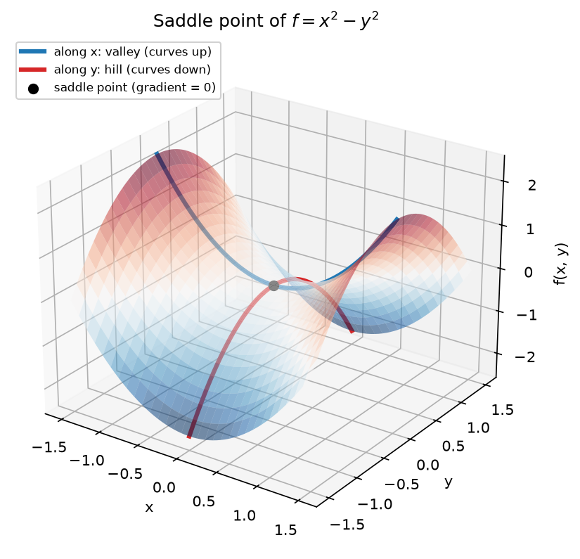
- ∇²𝑓(𝑥) ― the Hessian (Hessian matrix). The matrix whose (𝑖, 𝑗) element is ∂²𝑓/∂𝑥ᵢ∂𝑥ⱼ ; it describes the local curvature of the function. In computational chemistry, this Hessian is what is computed when normal mode frequencies of a molecule are obtained in a vibrational (frequency) calculation (strictly speaking, the mass-weighted version). Around a local minimum the function looks like a valley that curves upward in every direction, and around a local maximum it is a hill that curves downward in every direction. There are also points that look like a hill from one direction and like a valley from another; these are called saddle points (Figure 1). The transition state of a chemical reaction is exactly such a saddle point: a hill along the direction in which the reaction proceeds, and a valley in all other directions.
A necessary condition for 𝑥⋆ to be a local minimum is that the gradient is “zero” there:
∇f(x⋆) = 0.
At a point where the gradient is not zero, moving slightly in the direction opposite to the gradient lowers the function value, so the point is not a local minimum (Figure 2).
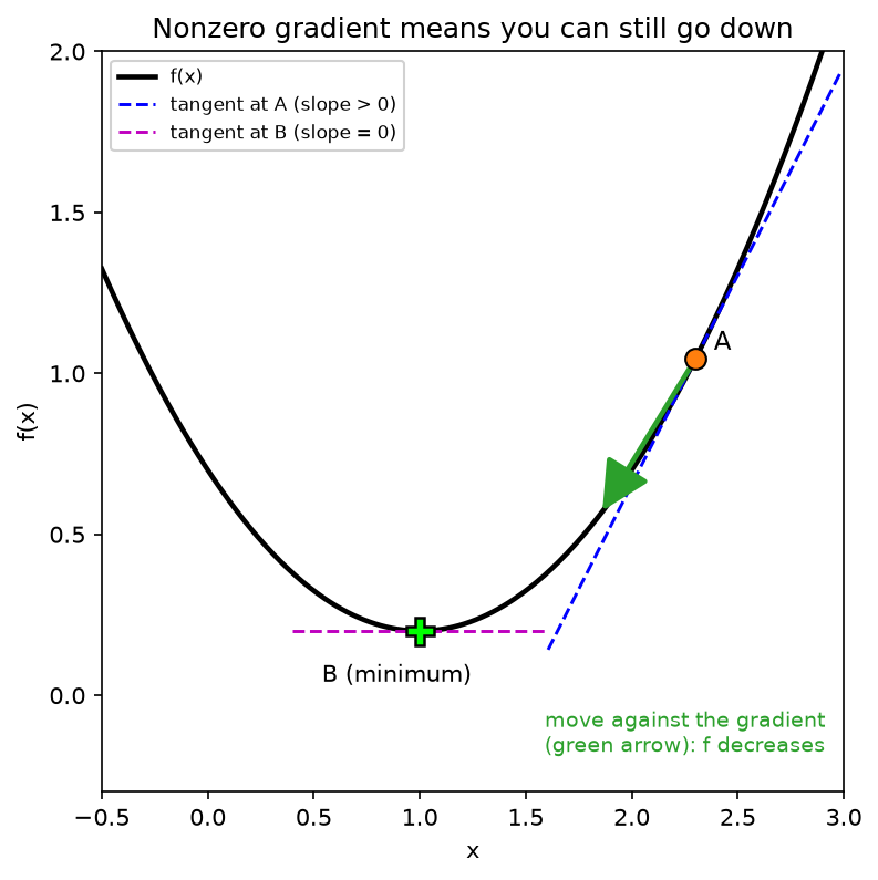
Furthermore, if in addition to zero gradient the Hessian describes a valley, the point is a local minimum. In the language of structure optimization, “the force on every atom is zero” is the necessary condition, and “no imaginary frequencies in the vibrational calculation” corresponds to confirming that the point is a minimum.
Many continuous optimization algorithms are designed around the problem of “finding a point where the gradient is zero,” and differ in how many orders of the Taylor expansion they use.
Convergence criterion used in the demos
In all the demos below, we use the same convergence criterion: “stop when the largest absolute value of the gradient components is less than 0.01.” Since we are looking for a point where the gradient is zero, we stop once the gradient has become small enough.
This is the same idea as the criterion commonly used in structure optimization in computational chemistry. For example, ASE uses “the largest force acting on any atom is less than fmax” as its convergence criterion. In machine learning training, on the other hand, one may instead repeat the update a fixed number of times, or stop when the loss on validation data stops improving.
Steepest Descent (Gradient Descent)
The most basic algorithm: from the point 𝑥ₖ, move in the direction opposite to the gradient.
xk+1 = xk − α∇f(xk),
where 𝛼 > 0 is the step size, also called the “learning rate” in machine learning. In the language of structure optimization, it is the simplest possible method: “move each atom a little in the direction of the force acting on it”; in the language of machine learning, “move the parameters a little in the direction that decreases the loss.”
The gradient is “the direction in which the function increases most steeply,” so its opposite is “the direction in which it decreases most steeply.” As long as we move only a little, going against the gradient is the most efficient way to lower the function value.
An example where steepest descent works
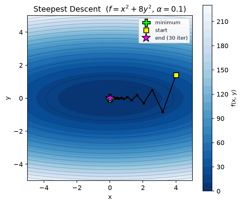
We minimize the quadratic function 𝑓(𝑥, 𝑦) = 𝑥² + 8𝑦², which has a long, narrow valley, from the initial point (4.0, 1.4) with 𝛼 = 0.1. Figure 3 shows the result: it reaches the minimum in 30 steps.
The difficulty with steepest descent
Looking at Figure 3, you can see that in the later iterations the update per step becomes small and convergence is slow. Why does this happen? It comes from two difficulties: “the shape of the function (its condition number)” and “the choice of the step size 𝛼.”
In this function, the curvature in the 𝑦 direction is 8 times that in the 𝑥 direction (the eigenvalues of the Hessian are 2 and 16). This “ratio of the curvature in the steepest direction to that in the flattest direction” is called the condition number. When the condition number is large, the valley becomes long and narrow, and the gradient vector points toward the valley walls rather than toward the valley floor. As a result, the method oscillates in the strongly curved 𝑦 direction and advances only slowly in the weakly curved 𝑥 direction.
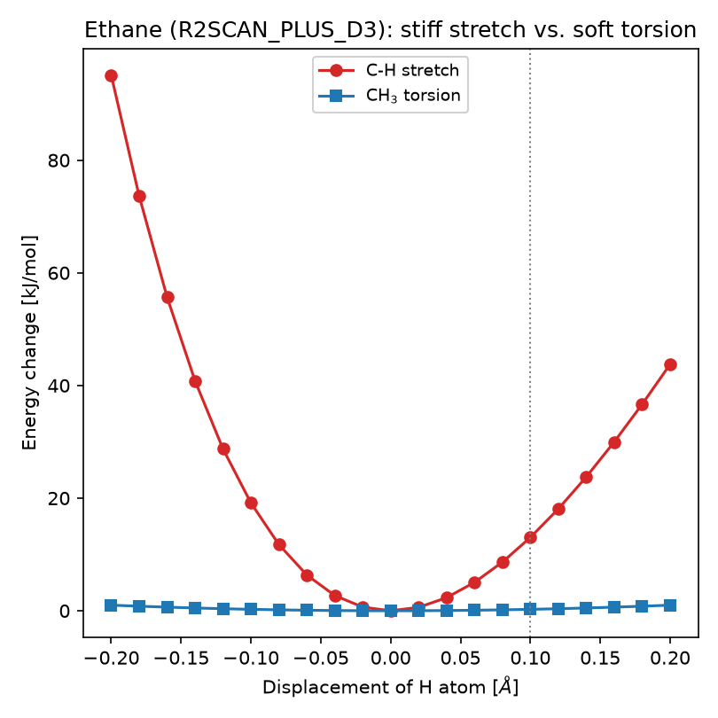
A large condition number is a problem frequently encountered in structure optimization of real molecules as well. Molecules contain both stiff bond stretches (large curvature) and soft torsions (small curvature), so their condition numbers tend to be large. For example, calculating ethane (CH₃–CH₃) with Matlantis PFP v9 (R2SCAN_PLUS_D3 mode), stretching a C–H bond by 0.1 Å raises the energy by about 13 kJ/mol, whereas twisting a methyl group around the C–C bond so that its H atoms move by the same 0.1 Å raises it by only about 0.26 kJ/mol (Figure 4). For the same atomic displacement, the energy increase differs by a factor of about 50, and the curvature at the valley floor by a factor of about 60. The same situation arises in machine learning when features have very different scales, which is one reason why features are standardized before training.
An example where steepest descent fails
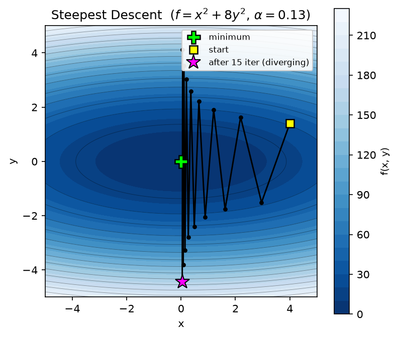
With the same function and the same initial point, we now run with a slightly larger step size, 𝛼 = 0.13. This time the optimization diverged (Figure 5). Because the step size was too large, in the strongly curved 𝑦 direction each step jumped over the valley, and each time it landed higher on the opposite slope.
Advantages and disadvantages of steepest descent
- Advantages: easy to implement. Works as long as the gradient is available.
- Disadvantages: choosing the step size 𝛼 is difficult. If 𝛼 is small, convergence is slow; if it is only slightly too large, the method can diverge.
Line Search — choosing the step size wisely
The difficulty with steepest descent was that “a good 𝛼 cannot be chosen in advance.” Line search is a technique that, after the search direction 𝑑ₖ has been decided, chooses how far to move along it (𝛼) at every step so that the function value decreases sufficiently.
The Armijo condition
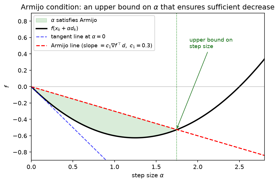
The most basic one is the Armijo condition: an 𝛼 that satisfies the following is accepted as “having decreased the function value sufficiently.”
f(xk + αdk) ≤ f(xk) + c1α∇f(xk)⊤dk, 0 < c1 < 1.
The right-hand side is a straight line whose slope is the slope at the starting point relaxed by a factor of 𝑐₁. The condition is passed if the actual function value lies below this line; intuitively, it “puts an upper limit on how far 𝛼 can be stretched.” A small value of about 10⁻⁴ is commonly used for 𝑐₁1. An 𝛼 satisfying this condition is found, for example, by backtracking: start from 𝛼 = 1 and keep halving 𝛼 until the condition is met.
The Wolfe conditions
With the Armijo condition alone, an extremely small 𝛼 also satisfies the condition, and progress can become slow. The Wolfe conditions are therefore widely used: in addition to the Armijo condition, they require that “at the new point, the slope is gentler than at the starting point.” The idea is that if the downhill slope is still steep, we should be able to go further, and this prevents 𝛼 from being too small. In formulas, the following is imposed in addition to the Armijo condition.
∇f(xk + αdk)⊤dk ≥ c2 ∇f(xk)⊤dk, 0 < c1 < c2 < 1.
The left-hand side is the slope at the new point, and the right-hand side is the slope at the starting point multiplied by 𝑐₂ ; on a downhill slope both are negative. This condition requires that the slope at the new point be sufficiently gentler than at the starting point, and it sets a lower limit on 𝛼.
If we also want to prevent going so far that we start climbing uphill, we use the strong Wolfe conditions, in which both sides are replaced by their absolute values.
|∇f(xk + αdk)⊤dk| ≤ c2|∇f(xk)⊤dk|.
For the quasi-Newton methods introduced in Part 2, 𝑐₁ = 10⁻⁴ and 𝑐₂ = 0.9 are typical 1.
Note that while the Armijo condition sets an upper limit on the step size, the additional part of the Wolfe conditions sets a lower limit. Therefore, backtracking that only shrinks the step size may fail to satisfy the Wolfe conditions. In practice, implementations instead search by shrinking the step if it is too long and extending it if it is too short.
Example: steepest descent + line search
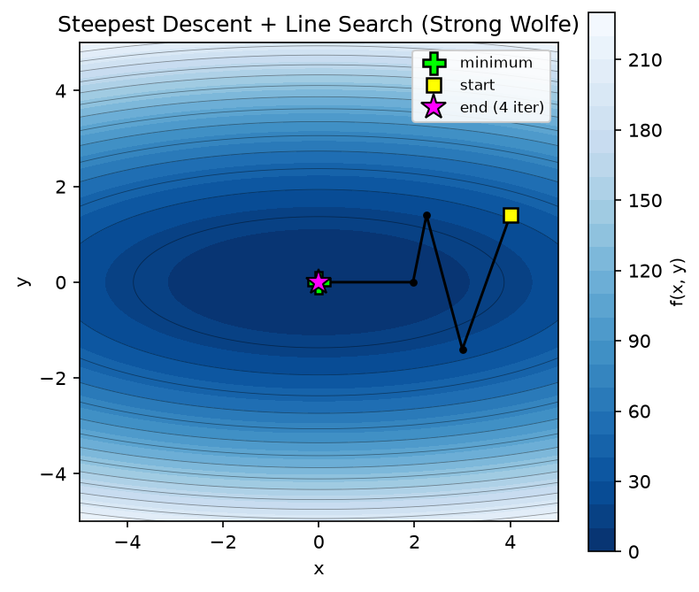
Figure 7 shows the result of steepest descent + line search (strong Wolfe conditions) with the same function and the same initial point. The optimization starts from the same point as in Figure 3, but because the step size is adjusted automatically at every iteration, the optimization that took 30 steps is shortened to 4 steps.
Line search is used not only with steepest descent but also in combination with many other methods, such as BFGS and L-BFGS introduced in Part 2. However, line search may evaluate the function value and gradient several times within a single step. When each energy and force evaluation is expensive, as in DFT, this additional cost cannot be ignored.
Newton’s Method
Steepest descent used only up to the first order (the gradient) of the Taylor expansion. Newton’s method uses up to the second order (the Hessian).
Using the second order, the function can be approximated by a quadratic function around the current point. Newton’s method jumps straight to the bottom of the valley of this approximating quadratic (we will see later what happens when the approximation is not a valley).
Let us first consider the case of a single variable. When we move from point x by d, the function value can be approximated by using the Taylor expansion up to second order:
f(x + d) ≈ f(x) + f ′(x) d + 12f ″(x) d2
The right-hand side is a quadratic function of d. At its bottom, the slope with respect to d is zero, so
f ′(x) + f ″(x) d = 0 ⇒ d = −f ′(x)f ″(x)
is the amount to move to reach the bottom of the approximating valley. In other words, it is “the slope” divided by “the curvature.” For the same slope, if the valley curves sharply (𝑓″ large), the bottom is close and we move only a little; if it curves gently (𝑓″ small), the bottom is far away and we move a lot.
With several variables, we replace the slope 𝑓′ by the gradient ∇𝑓 and the curvature 𝑓″ by the Hessian ∇²𝑓. “Dividing” by a matrix corresponds to multiplying by its inverse, so the step becomes
dk = −[∇2f(xk)]−1∇f(xk), xk+1 = xk + dk
Because the step is divided by the curvature direction by direction, the method moves cautiously along strongly curved directions and boldly along weakly curved ones, so the zigzag of steepest descent does not occur.
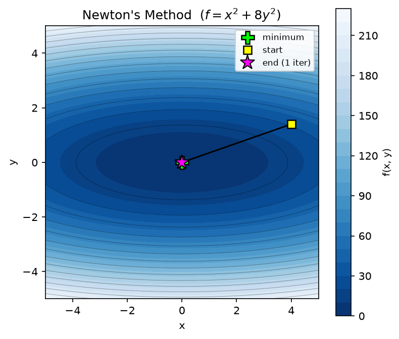
In regions where the function closely matches a quadratic locally, Newton’s method converges in far fewer iterations than steepest descent. In fact, if f is a valley-shaped quadratic function, Newton’s method reaches the exact solution in a single step.
An example where Newton’s method works
Figure 8 shows the result of optimizing the same 𝑓(𝑥, 𝑦) = 𝑥² + 8𝑦² with Newton’s method from the same initial point (4.0, 1.4). We can see that it reaches the solution in a single step.
An example where Newton’s method fails
Newton’s method only looks for “a point where the gradient is zero”; it does not distinguish whether that point is a local minimum, a local maximum, or a saddle point. If we make the second-order approximation in a hill-shaped region, the approximation is a “hill” rather than a “valley,” and Newton’s method jumps to the top of that hill. As an example, consider the following function, which has four local minima and a local maximum at the origin.
f(x, y) = 14(x4 + y4) − 12(x2 + y2)
The local minima are at (±1, ±1), and the region around the origin is hill-shaped. Running Newton’s method from the initial point (0.2, 0.15), it reaches the local maximum instead of a local minimum.
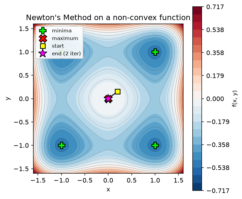
Since the gradient is zero at the origin, from the point of view of Newton’s method this is a “solution.” In fact, the Newton direction at this initial point points uphill, in the direction in which the function value increases.
Advantages and disadvantages of Newton’s method
- Advantages: in regions where the function is well approximated locally by a quadratic, it converges in very few iterations.
- Disadvantages: computing and storing the Hessian is expensive. In hill-shaped regions it may end up at a local maximum or a saddle point.
Summary of Part 1
In Part 1, we introduced steepest descent, line search, and Newton’s method. Steepest descent is a simple method that moves against the gradient and can be used as long as the gradient can be computed. On the other hand, too large a step size makes it diverge and too small a step size makes convergence slow, so choosing the step size matters. Line search chooses this step size automatically at every iteration and speeds up convergence considerably. However, the search direction is still the negative gradient. Newton’s method improves the direction itself by using the Hessian in addition to the gradient, and converges in very few iterations in regions that are well approximated by a quadratic. On the other hand, it has the drawbacks that “computing and storing the Hessian is expensive” and that “it may end up at a local maximum or a saddle point.” In Part 2, we introduce BFGS, which improves on Newton’s method by approximating the Hessian, and L-BFGS, which further reduces memory use for large-scale problems.
References
- Nocedal, J. & Wright, S. J. Numerical Optimization, 2nd ed. Springer, 2006.
- Umetani, S. Shikkari Manabu Suri Saitekika: Moderu kara Arugorizumu made [Mathematical Optimization: From Models to Algorithms]. Kodansha, 2020 (in Japanese).
- Kanamori, T., Suzuki, T., Takeuchi, I. & Sato, I. Kikai Gakushu no tame no Renzoku Saitekika [Continuous Optimization for Machine Learning] (Machine Learning Professional Series). Kodansha, 2016 (in Japanese).
-


 URL
Copied
New Articles
NEW
Matlantis and imec launch a joint development project on machine-learning simulation for nanoelectronics materials

Semiconductors Machine Learning Interatomic Potentials

NEW
How Do Materials Engineers in Japan View Computational Chemistry and Materials Informatics? – A survey of 82 R&D professionals reveals a gap that splits the field in two
Materials Informatics computational chemistry

The Lab Is (Not) All You Need: Why autonomous laboratories make atomistic simulation more valuable, not less

Lab Automation Machine Learning Interatomic Potentials

The front runner of AI for Science – A Report from the "Matlantis User Conference 2026"
Conference Report

Changing the rules of materials development with Physics-Grounded AI: how Matlantis PFP came to be

Interview